Modern Convolutional Networks

Data Mining Image

Introduction

Now that we understand the basics of wiring together CNNs, let’s take a tour of modern CNN architectures. This tour is, by necessity, incomplete, thanks to the plethora of exciting new designs being added.

Their importance derives from the fact that not only can they be used directly for vision tasks, but they also serve as basic feature generators for more advanced tasks such as

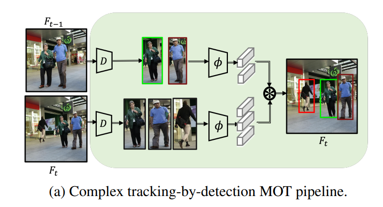
Tracking Zhang.Sun.Jiang.ea.2021.
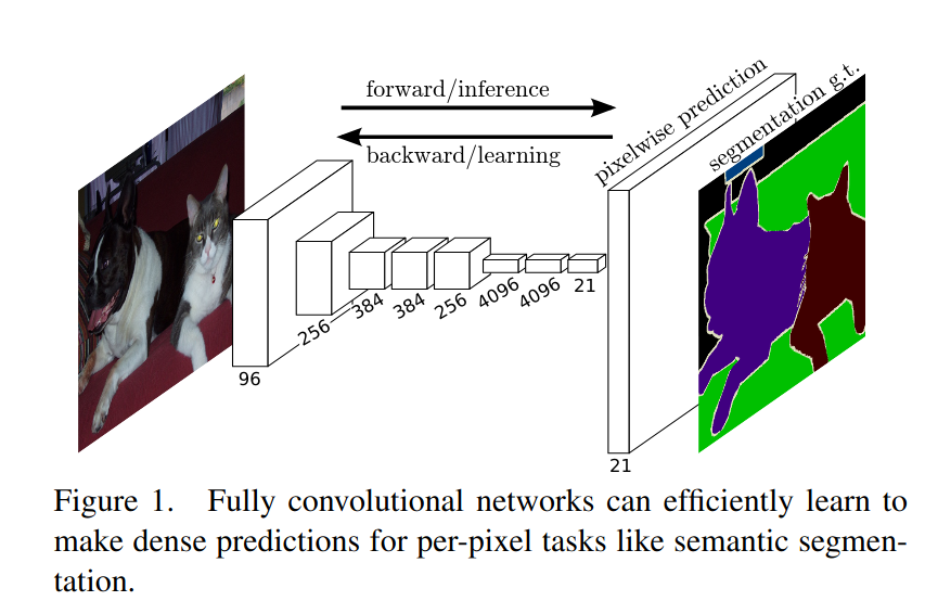
Segmentation Long.Shelhamer.Darrell.2015.
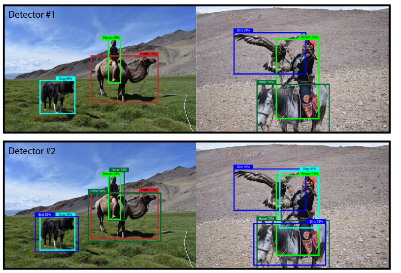
Object detection Redmon.Farhadi.2018
Style transformation Gatys.Ecker.Bethge.2016.

In this chapter, most sections correspond to a significant CNN architecture that was at some point (or currently) the base model upon which many research projects and deployed systems were built. Each of these networks was briefly a dominant architecture and many were winners or runners-up in the ImageNet competition which has served as a barometer of progress on supervised learning in computer vision since 2010. It is only recently that Transformers have begun to displace CNNs, starting with Dosovitskiy.Beyer.Kolesnikov.ea.2021 and followed by the Swin Transformer liu2021swin. We will cover this development later

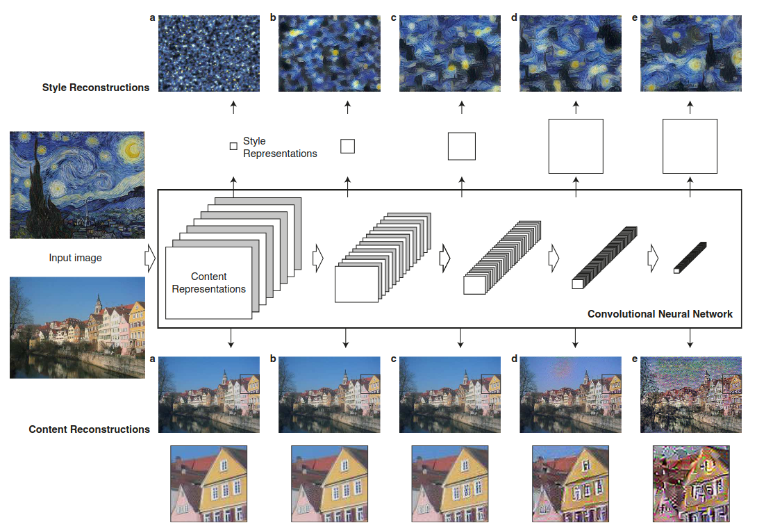
While the idea of deep neural networks is quite simple (stack together a bunch of layers), performance can vary wildly across architectures and hyperparameter choices. The neural networks described in this chapter are the product of intuition, a few mathematical insights, and a lot of trial and error. We present these models in chronological order, partly to convey a sense of the history so that you can form your own intuitions about where the field is heading and perhaps develop your own architectures. For instance, batch normalization and residual connections described in this chapter have offered two popular ideas for training and designing deep models, both of which have since also been applied to architectures beyond computer vision.

We begin our tour of modern CNNs with AlexNet Krizhevsky.Sutskever.Hinton.2012, the first large-scale network deployed to beat conventional computer vision methods on a large-scale vision challenge. The VGG network Simonyan.Zisserman.2014, which makes use of a number of repeating blocks of elements. The network in network (NiN) that convolves whole neural networks patch-wise over inputs Lin.Chen.Yan.2013. GoogLeNet that uses networks with multi-branch convolutions Szegedy.Liu.Jia.ea.2015, the residual network (ResNet) He.Zhang.Ren.ea.2016, which remains one of the most popular off-the-shelf architectures in computer vision; ResNeXt blocks Xie.Girshick.Dollar.ea.2017 for sparser connections; and DenseNet Huang.Liu.Van-Der-Maaten.ea.2017 for a generalization of the residual architecture. Over time many special optimizations for efficient networks have been developed, such as coordinate shifts (ShiftNet) wu2018shift]. This culminated in the automatic search for efficient architectures such as MobileNet v3 Howard.Sandler.Chu.ea.2019. It also includes the semi-automatic design exploration of that led to the RegNetX/Y which we will discuss later in this chapter. The work is instructive insofar as it offers a path for marrying brute force computation with the ingenuity of an experimenter in the search for efficient design spaces. Of note is also the work of as it shows that training techniques (e.g., optimizers, data augmentation, and regularization) play a pivotal role in improving accuracy. It also shows that long-held assumptions, such as the size of a convolution window, may need to be revisited, given the increase in computation and data.

We will cover this and many more questions in due course throughout this chapter.

Alex Net

Although CNNs were well known in the computer vision and machine learning communities following the introduction of LeNet LeCun.Jackel.Bottou.ea.1995, they did not immediately dominate the field. Although LeNet achieved good results on early small datasets, the performance and feasibility of training CNNs on larger, more realistic datasets had yet to be established. In fact, for much of the intervening time between the early 1990s and the watershed results of 2012 Krizhevsky.Sutskever.Hinton.2012, neural networks were often surpassed by other machine learning methods, such as kernel methods , ensemble methods, and structured estimation.

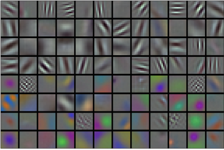
Representation for the 12 filters used by Alext Net

AlexNet, which employed an 8-layer CNN, won the ImageNet Large Scale Visual Recognition Challenge 2012 by a large margin. This network showed, for the first time, that the features obtained by learning can transcend manually-designed features, breaking the previous paradigm in computer vision.

Architecture of Lenet and Alex Net

In AlexNet’s first layer, the convolution window shape is $11\times11$. Since the images in ImageNet are eight times taller and wider than the MNIST images, objects in ImageNet data tend to occupy more pixels with more visual detail. Consequently, a larger convolution window is needed to capture the object. The convolution window shape in the second layer is reduced to $5\times5$, followed by $3\times3$. In addition, after the first, second, and fifth convolutional layers, the network adds max-pooling layers with a window shape of $3\times3$ and a stride of 2. Moreover, AlexNet has ten times more convolution channels than LeNet.

After the final convolutional layer, there are two huge fully connected layers with 4096 outputs. These layers require nearly 1GB model parameters. Because of the limited memory in early GPUs, the original AlexNet used a dual data stream design, so that each of their two GPUs could be responsible for storing and computing only its half of the model. Fortunately, GPU memory is comparatively abundant now, so we rarely need to break up models across GPUs these days (our version of the AlexNet model deviates from the original paper in this aspect).

Here is a possible definition of the model using pytorch.

class AlexNet(nn.Module):
        def __init__(self, lr=0.1, num_classes=10):
            super().__init__()
            self.save_hyperparameters()
            self.net = nn.Sequential(
                nn.LazyConv2d(96, kernel_size=11, stride=4, padding=1),
                nn.ReLU(), nn.MaxPool2d(kernel_size=3, stride=2),
                nn.LazyConv2d(256, kernel_size=5, padding=2), nn.ReLU(),
                nn.MaxPool2d(kernel_size=3, stride=2),
                nn.LazyConv2d(384, kernel_size=3, padding=1), nn.ReLU(),
                nn.LazyConv2d(384, kernel_size=3, padding=1), nn.ReLU(),
                nn.LazyConv2d(256, kernel_size=3, padding=1), nn.ReLU(),
                nn.MaxPool2d(kernel_size=3, stride=2), nn.Flatten(),
                nn.LazyLinear(4096), nn.ReLU(), nn.Dropout(p=0.5),
                nn.LazyLinear(4096), nn.ReLU(),nn.Dropout(p=0.5),
                nn.LazyLinear(num_classes))
            self.net.apply(d2l.init_cnn)

Networks using Blocks (VGG)

While AlexNet offered empirical evidence that deep CNNs can achieve good results, it did not provide a general template to guide subsequent researchers in designing new networks. In the following sections, we will introduce several heuristic concepts commonly used to design deep networks.

Progress in this field mirrors that of VLSI (very large scale integration) in chip design where engineers moved from placing transistors to logical elements to logic blocks. Similarly, the design of neural network architectures has grown progressively more abstract, with researchers moving from thinking in terms of individual neurons to whole layers, and now to blocks, repeating patterns of layers. A decade later, this has now progressed to researchers using entire trained models to repurpose them for different, albeit related, tasks. Such large pretrained models are typically called foundation models

Back to network design. The idea of using blocks first emerged from the Visual Geometry Group (VGG) at Oxford University, in their eponymously-named VGG network Simonyan.Zisserman.2014. It is easy to implement these repeated structures in code with any modern deep learning framework by using loops and subroutines.

VGG Blocks

The basic building block of CNNs is a sequence of the following:

A convolutional layer with padding to maintain the resolution.
A nonlinearity such as a ReLU.
A pooling layer such as max-pooling to reduce the resolution. One of the problems with this approach is that the spatial resolution decreases quite rapidly.

In particular, this imposes a hard limit of $\log_2 d$ convolutional layers on the network before all dimensions $d$ are used up. For instance, in the case of ImageNet, it would be impossible to have more than 8 convolutional layers in this way.

The key idea of Simonyan.Zisserman.2014 was to use multiple convolutions in between downsampling via max-pooling in the form of a block. They were primarily interested in whether deep or wide networks perform better. For instance, the successive application of two $3 \times 3$ convolutions touches the same pixels as a single $5 \times 5$ convolution does. At the same time, the latter uses approximately as many parameters $25 \cdot c^2$ as three $3 \times 3$ convolutions do $3 \cdot 9 \cdot c^2$. In a rather detailed analysis they showed that deep and narrow networks significantly outperform their shallow counterparts. This set deep learning on a quest for ever deeper networks with over 100 layers for typical applications. Stacking $3 \times 3$ convolutions has become a gold standard in later deep networks. Consequently, fast implementations for small convolutions have become a staple on GPUs.

Back to VGG: a VGG block consists of a sequence of convolutions with $3\times3$ kernels with padding of 1 (keeping height and width) followed by a $2 \times 2$ max-pooling layer with stride of 2 (halving height and width after each block). In the code below, we define a function called vgg_block to implement one VGG block.

    def vgg_block(num_convs, out_channels):
        layers = []
        for _ in range(num_convs):
            layers.append(nn.LazyConv2d(out_channels, kernel_size=3, padding=1))
            layers.append(nn.ReLU())
        layers.append(nn.MaxPool2d(kernel_size=2,stride=2))
        return nn.Sequential(*layers)

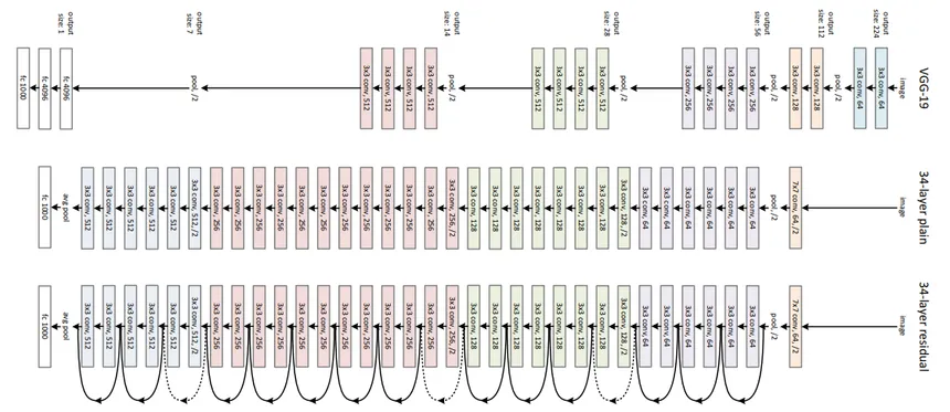
Like AlexNet and LeNet, the VGG Network can be partitioned into two parts: the first consisting mostly of convolutional and pooling layers and the second consisting of fully connected layers that are identical to those in AlexNet. The key difference is that the convolutional layers are grouped in nonlinear transformations that leave the dimensonality unchanged, followed by a resolution-reduction step, as depicted in the following figure:

Comparison between Alex Net and VGG Architecture.

The convolutional part of the network connects several VGG blocks(also defined in the vgg_block function) in succession. This grouping of convolutions is a pattern that has remained almost unchanged over the past decade, although the specific choice of operations has undergone considerable modifications. The variable arch consists of a list of tuples (one per block), where each contains two values: the number of convolutional layers and the number of output channels, which are precisely the arguments required to call the vgg_block function. As such, VGG defines a family of networks rather than just a specific manifestation. To build a specific network we simply iterate over arch to compose the blocks.

Here is the declaration using the pytorch pay a close attention to the arch argument.

class VGG(nn.Module):
    def __init__(self, arch, lr=0.1, num_classes=10):
        super().__init__()
        self.save_hyperparameters()
        conv_blks = []
        for (num_convs, out_channels) in arch:
            conv_blks.append(vgg_block(num_convs, out_channels))
        self.net = nn.Sequential(
            *conv_blks, nn.Flatten(),
            nn.LazyLinear(4096), nn.ReLU(), nn.Dropout(0.5),
            nn.LazyLinear(4096), nn.ReLU(), nn.Dropout(0.5),
            nn.LazyLinear(num_classes))
        self.net.apply(d2l.init_cnn)

The original VGG network had five convolutional blocks, among which the first two have one convolutional layer each and the latter three contain two convolutional layers each. The first block has 64 output channels and each subsequent block doubles the number of output channels, until that number reaches 512. Since this network uses eight convolutional layers and three fully connected layers, it is often called VGG-11.

VGG(arch=((1, 64), (1, 128), (2, 256), (2, 512), (2, 512)))

Network in Network

LeNet, AlexNet, and VGG all share a common design pattern: extract features exploiting spatial structure via a sequence of convolutions and pooling layers and post-process the representations via fully connected layers. The improvements upon LeNet by AlexNet and VGG mainly lie in how these later networks widen and deepen these two modules.

This design poses two major challenges.

First, the fully connected layers at the end of the architecture consume tremendous numbers of parameters. For instance, even a simple model such as VGG-11 requires a monstrous matrix, occupying almost 400MB of RAM in single precision (FP32). This is a significant impediment to computation, in particular on mobile and embedded devices. After all, even high-end mobile phones sport no more than 8GB of RAM. At the time VGG was invented, this was an order of magnitude less (the iPhone 4S had 512MB). As such, it would have been difficult to justify spending the majority of memory on an image classifier.
Second, it is equally impossible to add fully connected layers earlier in the network to increase the degree of nonlinearity: doing so would destroy the spatial structure and require potentially even more memory.

The network in network (NiN) blocks Lin.Chen.Yan.2013 offer an alternative, capable of solving both problems in one simple strategy. They were proposed based on a very simple insight:

Use $1 \times 1$ convolutions to add local nonlinearities across the channel activations.
Use global average pooling to integrate across all locations in the last representation layer. Note that global average pooling would not be effective, were it not for the added nonlinearities.

Lets’ dive into the details:

NiN Blocks

The idea behind NiN is to apply a fully connected layer at each pixel location (for each height and width). The resulting $1 \times 1$ convolution can be thought of as a fully connected layer acting independently on each pixel location.

The following figure illustrates the main structural differences between VGG and NiN, and their blocks. Note both the difference in the NiN blocks (the initial convolution is followed by $1 \times 1$ convolutions, whereas VGG retains $3 \times 3$ convolutions) and at the end where we no longer require a giant fully connected layer.

Comparison between Alex Net, VGG and Network in Networks.

Here is the code for a NiN block

def nin_block(out_channels, kernel_size, strides, padding):
    return nn.Sequential(
        nn.LazyConv2d(out_channels, kernel_size, strides, padding), nn.ReLU(),
        nn.LazyConv2d(out_channels, kernel_size=1), nn.ReLU(),
        nn.LazyConv2d(out_channels, kernel_size=1), nn.ReLU())

NiN Model

NiN uses the same initial convolution sizes as AlexNet (it was proposed shortly thereafter). The kernel sizes are $11\times 11$, $5\times 5$, and $3\times 3$, respectively, and the numbers of output channels match those of AlexNet. Each NiN block is followed by a max-pooling layer with a stride of 2 and a window shape of $3\times 3$.

The second significant difference between NiN and both AlexNet and VGG is that NiN avoids fully connected layers altogether. Instead, NiN uses a NiN block with a number of output channels equal to the number of label classes, followed by a global average pooling layer, yielding a vector of logits. This design significantly reduces the number of required model parameters, albeit at the expense of a potential increase in training time.

Here is the definition of the model in pytorch.

class NiN(nn.Module):
    def __init__(self, lr=0.1, num_classes=10):
        super().__init__()
        self.save_hyperparameters()
        self.net = nn.Sequential(
            nin_block(96, kernel_size=11, strides=4, padding=0),
            nn.MaxPool2d(3, stride=2),
            nin_block(256, kernel_size=5, strides=1, padding=2),
            nn.MaxPool2d(3, stride=2),
            nin_block(384, kernel_size=3, strides=1, padding=1),
            nn.MaxPool2d(3, stride=2),
            nn.Dropout(0.5),
            nin_block(num_classes, kernel_size=3, strides=1, padding=1),
            nn.AdaptiveAvgPool2d((1, 1)),
            nn.Flatten())
        self.net.apply(d2l.init_cnn)

Multi-Branch Networks (GoogLeNet)

In 2014, GoogLeNet won the ImageNet Challenge Szegedy.Liu.Jia.ea.2015, using a structure that combined the strengths of NiN , repeated blocks, and a cocktail of convolution kernels. It was arguably also the first network that exhibited a clear distinction among the stem (data ingest), body (data processing), and head (prediction) in a CNN. This design pattern has persisted ever since in the design of deep networks: the stem is given by the first two or three convolutions that operate on the image. They extract low-level features from the underlying images. This is followed by a body of convolutional blocks. Finally, the head maps the features obtained so far to the required classification, segmentation, detection, or tracking problem at hand.

The key contribution in GoogLeNet was the design of the network body. It solved the problem of selecting convolution kernels in an ingenious way. While other works tried to identify which convolution, ranging from $1 \times 1$ to $11 \times 11$ would be best, it simply concatenated multi-branch convolutions. In what follows we introduce a slightly simplified version of GoogLeNet: the original design included a number of tricks for stabilizing training through intermediate loss functions, applied to multiple layers of the network. They are no longer necessary due to the availability of improved training algorithms.

Inception Blocks

The basic convolutional block in GoogLeNet is called an Inception block, stemming from the meme “need to go deeper” from the movie Inception.

Structure of the Inception block.

As depicted in the previous figure, the inception block consists of four parallel branches. The first three branches use convolutional layers with window sizes of $1\times 1$, $3\times 3$, and $5\times 5$ to extract information from different spatial sizes. The middle two branches also add a $1\times 1$ convolution of the input to reduce the number of channels, reducing the modelss complexity. The fourth branch uses a $3\times 3$ max-pooling layer, followed by a $1\times 1$ convolutional layer to change the number of channels. The four branches all use appropriate padding to give the input and output the same height and width. Finally, the outputs along each branch are concatenated along the channel dimension and comprise the block’s output. The commonly-tuned hyperparameters of the Inception block are the number of output channels per layer, i.e., how to allocate capacity among convolutions of different size.

To gain some intuition for why this network works so well, consider the combination of the filters. They explore the image in a variety of filter sizes. This means that details at different extents can be recognized efficiently by filters of different sizes. At the same time, we can allocate different amounts of parameters for different filters.

Here is the code to implement this block:

class Inception(nn.Module):
    # c1--c4 are the number of output channels for each branch
    def __init__(self, c1, c2, c3, c4, **kwargs):
        super(Inception, self).__init__(**kwargs)
        # Branch 1
        self.b1_1 = nn.LazyConv2d(c1, kernel_size=1)
        # Branch 2
        self.b2_1 = nn.LazyConv2d(c2[0], kernel_size=1)
        self.b2_2 = nn.LazyConv2d(c2[1], kernel_size=3, padding=1)
        # Branch 3
        self.b3_1 = nn.LazyConv2d(c3[0], kernel_size=1)
        self.b3_2 = nn.LazyConv2d(c3[1], kernel_size=5, padding=2)
        # Branch 4
        self.b4_1 = nn.MaxPool2d(kernel_size=3, stride=1, padding=1)
        self.b4_2 = nn.LazyConv2d(c4, kernel_size=1)

    def forward(self, x):
        b1 = F.relu(self.b1_1(x))
        b2 = F.relu(self.b2_2(F.relu(self.b2_1(x))))
        b3 = F.relu(self.b3_2(F.relu(self.b3_1(x))))
        b4 = F.relu(self.b4_2(self.b4_1(x)))
        return torch.cat((b1, b2, b3, b4), dim=1)

GoogLeNet Model

As shown in following figure, GoogLeNet uses a stack of a total of 9 inception blocks, arranged into three groups with max-pooling in between, and global average pooling in its head to generate its estimates. Max-pooling between inception blocks reduces the dimensionality. At its stem, the first module is similar to AlexNet and LeNet.

The GoogLeNet architecture.

We can now implement GoogLeNet piece by piece. Letss begin with the stem. The first module uses a 64-channel :math:7\times 7 convolutional layer.

class GoogleNet(nn.Module):
    def b1(self):
        return nn.Sequential(
            nn.LazyConv2d(64, kernel_size=7, stride=2, padding=3),
            nn.ReLU(), nn.MaxPool2d(kernel_size=3, stride=2, padding=1))

The second module uses two convolutional layers: first, a 64-channel $1\times 1$ convolutional layer, followed by a $3\times 3$ convolutional layer that triples the number of channels. This corresponds to the second branch in the Inception block and concludes the design of the body. At this point we have 192 channels.

def b2(self):
    return nn.Sequential(
        nn.LazyConv2d(64, kernel_size=1), nn.ReLU(),
        nn.LazyConv2d(192, kernel_size=3, padding=1), nn.ReLU(),
        nn.MaxPool2d(kernel_size=3, stride=2, padding=1))

The third module connects two complete Inception blocks in series. The number of output channels of the first Inception block is $64+128+32+32=256$. This amounts to a ratio of the number of output channels among the four branches of $2:4:1:1$. To achieve this, we first reduce the input dimensions by $\frac{1}{2}$ and by $\frac{1}{12}$ in the second and third branch respectively to arrive at $96 = 192/2$ and $16 = 192/12$ channels respectively.

The number of output channels of the second Inception block is increased to $128+192+96+64=480$, yielding a ratio of $128:192:96:64 = 4:6:3:2$. As before, we need to reduce the number of intermediate dimensions in the second and third channel. A scale of $\frac{1}{2}$ and $\frac{1}{8}$ respectively suffices, yielding $128$ and $32$ channels respectively. This is captured by the arguments of the following Inception block constructors.

def b3(self):
    return nn.Sequential(Inception(64, (96, 128), (16, 32), 32),
                         Inception(128, (128, 192), (32, 96), 64),
                         nn.MaxPool2d(kernel_size=3, stride=2, padding=1))

The fourth module is more complicated. It connects five Inception blocks in series, and they have $192+208+48+64=512$, $160+224+64+64=512$, $128+256+64+64=512$ $112+288+64+64=528$, and $256+320+128+128=832$ output channels, respectively. The number of channels assigned to these branches is similar to that in the third module: the second branch with the $3\times 3$ convolutional layer outputs the largest number of channels, followed by the first branch with only the $1\times 1$ convolutional layer, the third branch with the $5\times 5$ convolutional layer, and the fourth branch with the $3\times 3$ max-pooling layer. The second and third branches will first reduce the number of channels according to the ratio. These ratios are slightly different in different Inception blocks.

def b4(self):
    return nn.Sequential(Inception(192, (96, 208), (16, 48), 64),
                         Inception(160, (112, 224), (24, 64), 64),
                         Inception(128, (128, 256), (24, 64), 64),
                         Inception(112, (144, 288), (32, 64), 64),
                         Inception(256, (160, 320), (32, 128), 128),
                         nn.MaxPool2d(kernel_size=3, stride=2, padding=1))

The fifth module has two Inception blocks with $256+320+128+128=832$ and $384+384+128+128=1024$ output channels. The number of channels assigned to each branch is the same as that in the third and fourth modules, but differs in specific values. It should be noted that the fifth block is followed by the output layer. This block uses the global average pooling layer to change the height and width of each channel to 1, just as in NiN. Finally, we turn the output into a two-dimensional array followed by a fully connected layer whose number of outputs is the number of label classes.

def b5(self):
    return nn.Sequential(Inception(256, (160, 320), (32, 128), 128),
                         Inception(384, (192, 384), (48, 128), 128),
                         nn.AdaptiveAvgPool2d((1,1)), nn.Flatten())