Course overview

Basic Machine Learning

Machine Learning as Data-Driven Programming

Machine Learning (ML) is fundamentally a form of data-driven programming. Unlike traditional programming, where a human explicitly defines the rules and logic to solve a problem, machine learning leverages data to automatically discover patterns and relationships. This approach is particularly powerful when dealing with complex tasks that are difficult to code manually, such as recognizing objects in images, translating languages, or predicting future trends.

One illustrative example of data-driven programming is the Optical Character Recognition (OCR) problem, specifically the classification of handwritten digits. Imagine you are tasked with developing a system that can recognize and classify digits (0-9) written by different people. Manually defining rules for every possible way someone might write a “7” or “5” is impractical due to the immense variability in handwriting styles. Instead, with machine learning, we can train a model to learn these patterns from data.

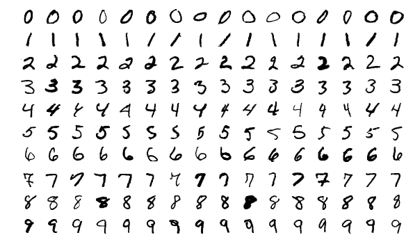
A well-known dataset used to tackle this problem is the MNIST dataset, which consists of 60,000 training images and 10,000 test images of handwritten digits. Each image is a 28x28 pixel grayscale image, and the task is to classify each image into one of the 10 digit classes.

AlexNet 2012 Paper by Alex Krizhevsky, Ilya Sutskever, and Geoffrey Hinton
MNIST Dataset

In this scenario, machine learning models are trained on the labeled data from the MNIST dataset, learning to associate pixel patterns with specific digits. Once trained, these models can generalize to accurately classify new, unseen images of digits, effectively automating the OCR task.

This example highlights the essence of machine learning: creating algorithms that learn from data rather than being explicitly programmed, making it possible to solve complex problems in an efficient and scalable manner.

Elements of an ML Algorithm

The (supervised) machine learning approach involves collecting a training set of images with known labels. These labeled images are then fed into a machine learning algorithm, which will (if done well), automatically produce a “program” that solves the task.

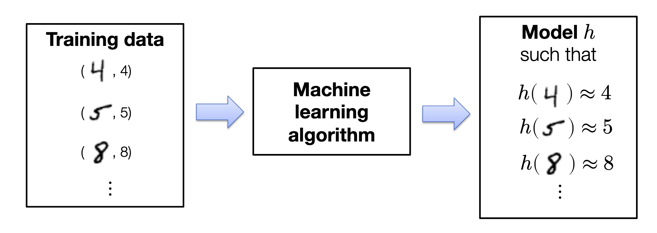
Every machine learning algorithm consists of three different elements:

Hypothesis Class

In the context of machine learning, the hypothesis class refers to the set of all possible functions or models that the algorithm can choose from to map inputs (such as images of digits) to outputs (like class labels or probabilities of different class labels). This “program structure” is defined by a set of parameters that the algorithm will learn during the training process.

Think of the hypothesis class as a blueprint for building the model. It defines the general form or structure that the final model will take, but not the specific details. For example, in a simple linear classifier, the hypothesis class might include all possible straight lines that can separate different classes of data points. The exact line chosen will depend on the parameters that are learned from the data.

The flexibility of the hypothesis class is crucial

• it determines the types of patterns the model can learn.
• A more complex hypothesis class might allow the model to capture more intricate relationships in the data, but it also risks overfitting (learning the noise instead of the true signal).

Thus, choosing the right hypothesis class is a balance between flexibility and simplicity.

Example 1: Linear Classifier Hypothesis Class

In a linear classifier, the hypothesis class consists of all possible linear functions that can separate different digit classes. For instance, suppose you have two-dimensional features extracted from the digit images (e.g., pixel intensity and another feature). The linear classifier would attempt to find a straight line (or a hyperplane in higher dimensions) that separates one digit class from another.

• Simple Hypothesis Class: Here, the hypothesis class is restricted to straight lines. This simplicity makes it easier to learn from the data, but it also means that the classifier can only correctly classify the digits if they are linearly separable—if the digits can be distinguished by a straight line or boundary in the feature space. For example, it might work well for distinguishing between digits like “1” and “7,” where the distinguishing feature might be as simple as a vertical stroke versus a slanted stroke.

Example 2: Neural Network Hypothesis Class

In contrast, consider a neural network as your hypothesis class. Neural networks, especially deep ones, have a much more complex hypothesis class because they consist of multiple layers of neurons that can capture non-linear relationships between input features.

• Complex Hypothesis Class: Here, the hypothesis class includes a vast range of non-linear functions. This flexibility allows the model to capture intricate patterns and relationships in the data that a linear classifier would miss. For instance, a neural network could easily distinguish between digits like “8” and “3,” which have complex curves and loops, by learning non-linear boundaries in the feature space. The complexity of the hypothesis class allows the network to adapt to the subtle variations in handwriting styles, curvature, and orientation that might be present in the digits.

Summary

These two examples highlight how the hypothesis class can vary significantly:

• A linear classifier represents a simple hypothesis class, with limitations in capturing complex patterns but is easier to train and interpret.
• A neural network represents a complex hypothesis class, capable of learning more intricate relationships but requiring more data and computational resources to train effectively.

The choice between these two (or other) hypothesis classes depends on the problem at hand, the complexity of the data, and the resources available for training.

Loss Function

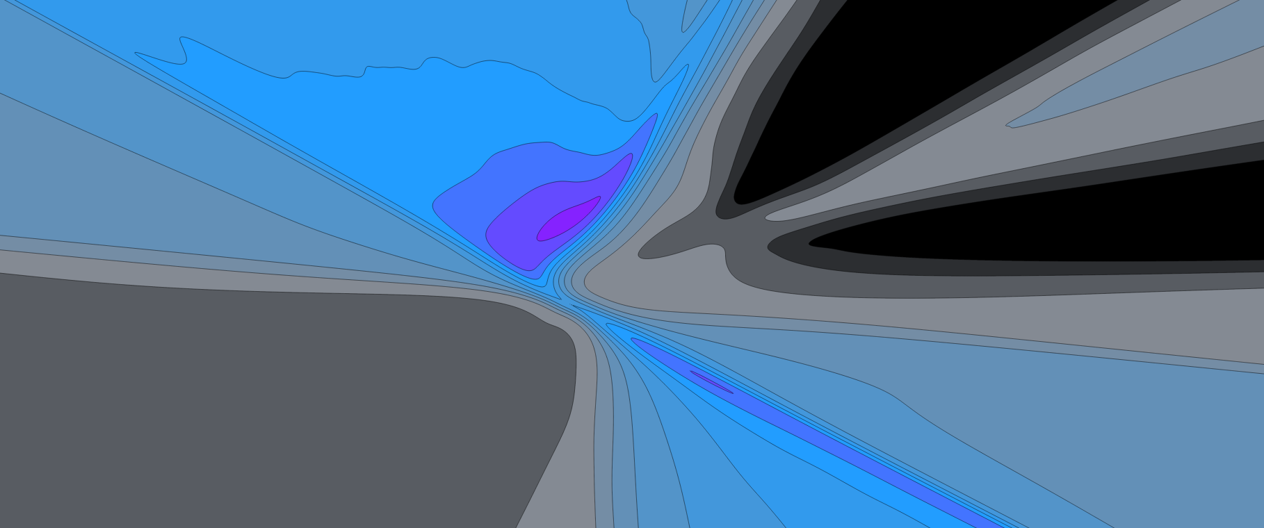
Visualizing the loss function of neural network
Visualizing the landscape of loss function for neural networks

The loss function is a crucial component of any machine learning algorithm. It acts as a measure of error or discrepancy between the model’s predictions and the actual labels in the training data. In essence, the loss function quantifies how well or poorly the model is performing at any given point during training.

The goal of the machine learning algorithm is to find the set of parameters in the hypothesis class that minimizes this loss function. By minimizing the loss, the model becomes more accurate in making predictions on new, unseen data.

Loss Function 1 : Classification Error

The simplest loss function to use in classification is just the Classification error. Which simply translates if the classifier has made an error or not

• We typically use this loss to assess the quality of the classifier.

Unfortunately, this error is a bad loss function to use for optimisation. Because it’s not differentiable.

Loss Function 2 : Cross Entropy

We will use a more adequate loss function Softmax or Cross Entropy which will exponentiate the entries of the hypothesis function (H) and then normalize the entries to make them sum to one.

Then we define the loss as the negative log probability of the true class.

Optimization Goal:

The third ingredient of a machine learning algorithm is a method to solve the associated optimisation problem. i.e the problem of minimizing the average loss on the training set:

For our linear Classifier Model, you will minimize the following problem:

One classical method it to use Gradient Descent which needs to compute the Gradient of the loss function.

• Advanced Optimizers: There are more sophisticated variants of gradient descent, like Adam, RMSprop, and Adagrad, which adaptively adjust the learning rate and incorporate momentum, allowing for faster and more reliable convergence. These optimizers are especially useful in training deep neural networks where the optimization landscape can be complex.

For our linear Classifier, where the hyptothesis is defined as $f: \mathbb{R}^{n\times k}\rightarrow \mathbb{R}$, the gradient is defined as the Matrix of Partial derivatives

And to minimize the function, the gradient descent algorithm proceeds by iteratively taking steps in the direction of the negative gradient

Where $\alpha$ is the step size. The following figure shows the evolution of the algorithms with different steps sizes.

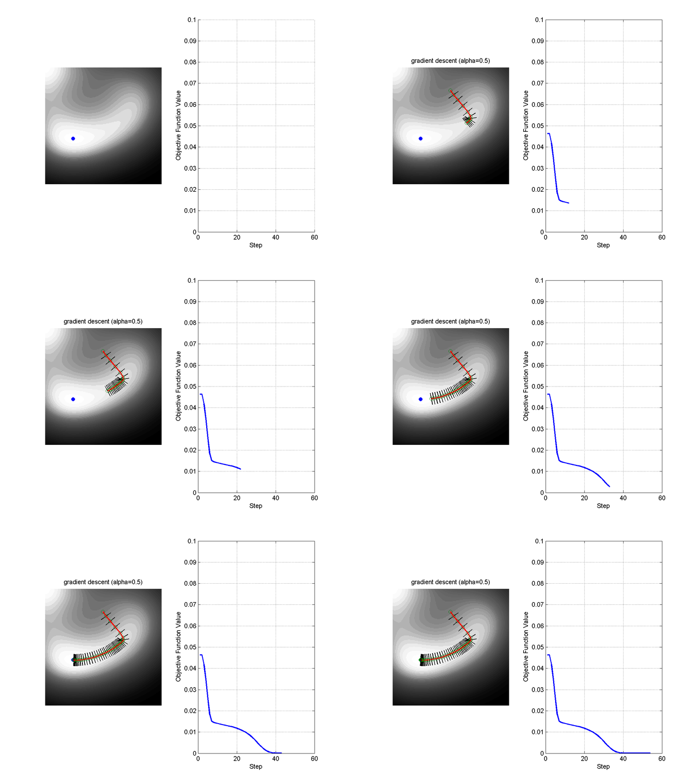
Figure: Comparison of Gradient Descent with Step Size 0.1 (left) and Step Size 0.5 (right).

The objective of the machine learning algorithm is to minimize the loss function across all examples in the training set. During training, the algorithm adjusts the parameters of the model to reduce the loss, thereby improving the model’s predictions. The process of minimizing the loss function is what ultimately allows the model to generalize well to new, unseen data.

Stochastic Gradient Descent

If our objective ( as in the case of Machine learning) is the sum of individual losses, we don’t want to compute the gradient using all examples to make a single update to the parameters.

Repeat:

• Sample a mini-batch of Data $X\in \mathbb{R}^{B\times n}$ and $y\in (1,\ldots, k)^B$
• Update the parameters using the Batch Gradient:

Gradient Cross Entropy

Now we will move our attention to compute the gradient of the cross entropy loss function?

Generally this done using Backpropagration that we will cover in more details in next chapters.

So let’s start by computing the gradient of the soft max function itself to a general vector $h\in\mathbb{R}^k$

The expression below could be written in Vector Form as

Where $z$ is the normalisation of the vector $\exp(h)$.

Now we will move the hard part where we need to compute the gradient for the full loss.

We will use the chain rule of multivariate calculus. But we need to be careful of the all the matrices dimensions.

The above formula is wrong as the dimension of the gradient is $(n\times k)$ while the provided formula has a dimension $k\times n$. The correct formula is

Now you are setup to implement a linear classifier for Image classification. As we will dive deeper in the course of Neural Network, we will explore more fancier hypothesis.