Multi Layers Perceptrons

Introduction

Previously, we introduced Softmax classification, implementing the algorithm from scratch. This allowed us to train classifiers capable of recognizing 10 categories of objects from low-resolution images. Along the way, we learned how to wrangle data, coerce our outputs into a valid probability distribution, apply an appropriate loss function, and minimize it with respect to our model’s parameters. Now that we have mastered these mechanics in the context of simple linear models, we can launch our exploration of deep neural networks, the comparatively rich class of models with which this book is primarily concerned.

Hidden Layers

We described affine transformations in as linear transformations with added bias. To begin, recall the model architecture corresponding to our softmax classification example. This model maps inputs directly to outputs via a single affine transformation, followed by a softmax operation. If our labels truly were related to the input data by a simple affine transformation, then this approach would be sufficient. However, linearity (in affine transformations) is a strong assumption.

Limitations of Linear Models

For example, linearity implies the weaker assumption of monotonicity, i.e., that any increase in our feature must either always cause an increase in our models output (if the corresponding weight is positive), or always cause a decrease in our modelss output (if the corresponding weight is negative). Sometimes that makes sense. For example, if we were trying to predict whether an individual will repay a loan, we might reasonably assume that all other things being equal, an applicant with a higher income would always be more likely to repay than one with a lower income. While monotonic, this relationship likely is not linearly associated with the probability of repayment. An increase in income from 0 to 50,000 likely corresponds to a bigger increase in likelihood of repayment than an increase from 1 million to 1.05 million. One way to handle this might be to postprocess our outcome such that linearity becomes more plausible, by using the logistic map (and thus the logarithm of the probability of outcome).

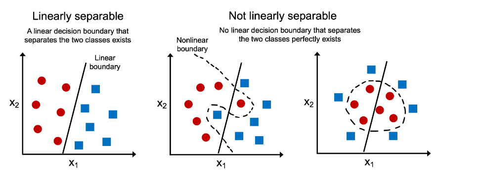
Note that we can easily come up with examples that violate monotonicity. Say for example that we want to predict health as a function of body temperature. For individuals with a normal body temperature above 37°C, higher temperatures indicate greater risk. However, if the body temperatures drops below 37°C, lower temperatures indicate greater risk! Again, we might resolve the problem with some clever preprocessing, such as using the distance from 37°C as a feature.

But what about classifying images of cats and dogs? Should increasing the intensity of the pixel at location (13, 17) always increase (or always decrease) the likelihood that the image depicts a dog? Reliance on a linear model corresponds to the implicit assumption that the only requirement for differentiating cats and dogs is to assess the brightness of individual pixels.

This approach is doomed to fail in a world where inverting an image preserves the category.

And yet despite the apparent absurdity of linearity here, as compared with our previous examples, it is less obvious that we could address the problem with a simple preprocessing fix. That is, because the significance of any pixel depends in complex ways on its context (the values of the surrounding pixels). While there might exist a representation of our data that would take into account the relevant interactions among our features, on top of which a linear model would be suitable, we simply do not know how to calculate it by hand. With deep neural networks, we used observational data to jointly learn both a representation via hidden layers and a linear predictor that acts upon that representation.

This problem of nonlinearity has been studied for at least a century Fisher.1928. For instance, decision trees in their most basic form use a sequence of binary decisions to decide upon class membership. Likewise, kernel methods have been used for many decades to model nonlinear dependencies Aronszajn.1950. This has found its way into nonparametric spline models and kernel methods Scholkopf.Smola.2002. It is also something that the brain solves quite naturally.

Incorporating Hidden Layers

We can overcome the limitations of linear models by incorporating one or more hidden layers. The easiest way to do this is to stack many fully connected layers on top of one another. Each layer feeds into the layer above it, until we generate outputs. We can think of the first $L-1$ layers as our representation and the final layer as our linear predictor. This architecture is commonly called a multilayer perceptron, often abbreviated as MLP.

An MLP with a hidden layer of five hidden units.

This MLP has four inputs, three outputs, and its hidden layer contains five hidden units. Since the input layer does not involve any calculations, producing outputs with this network requires implementing the computations for both the hidden and output layers. Thus, the number of layers in this MLP is two. Note that both layers are fully connected. Every input influences every neuron in the hidden layer, and each of these in turn influences every neuron in the output layer. Alas, we are not quite done yet.

From Linear to Nonlinear

As before, we denote by the matrix $\mathbf{X} \in \mathbb{R}^{n \times d}$ a minibatch of $n$ examples where each example has $d$ inputs (features). For a one-hidden-layer MLP whose hidden layer has $h$ hidden units, we denote by $\mathbf{H} \in \mathbb{R}^{n \times h}$ the outputs of the hidden layer, which are hidden representations. Since the hidden and output layers are both fully connected, we have hidden-layer weights $\mathbf{W}^{(1)} \in \mathbb{R}^{d \times h}$ and biases $\mathbf{b}^{(1)} \in \mathbb{R}^{1 \times h}$ and output-layer weights $\mathbf{W}^{(2)} \in \mathbb{R}^{h \times q}$ and biases $\mathbf{b}^{(2)} \in \mathbb{R}^{1 \times q}$. This allows us to calculate the outputs $\mathbf{O} \in \mathbb{R}^{n \times q}$ of the one-hidden-layer MLP as follows:

Note that after adding the hidden layer, our model now requires us to track and update additional sets of parameters. So what have we gained in exchange? You might be surprised to find out that’s in the model defined above we gain nothing for our troubles The reason is plain. The hidden units above are given by an affine function of the inputs, and the outputs (pre-softmax) are just an affine function of the hidden units. An affine function of an affine function is itself an affine function. Moreover, our linear model was already capable of representing any affine function.

To see this formally we can just collapse out the hidden layer in the above definition, yielding an equivalent single-layer model with parameters $\mathbf{W} = \mathbf{W}^{(1)}\mathbf{W}^{(2)}$ and $\mathbf{b} = \mathbf{b}^{(1)} \mathbf{W}^{(2)} + \mathbf{b}^{(2)}$:

In order to realize the potential of multilayer architectures, we need one more key ingredient: a nonlinear activation function $\sigma$ to be applied to each hidden unit following the affine transformation. For instance, a popular choice is the ReLU (rectified linear unit) activation function Nair.Hinton.2010 $\sigma(x) = \mathrm{max}(0, x)$ operating on its arguments elementwise. The outputs of activation functions $\sigma(\cdot)$ are called activations. In general, with activation functions in place, it is no longer possible to collapse our MLP into a linear model:

Since each row in $\mathbf{X}$ corresponds to an example in the minibatch, with some abuse of notation, we define the nonlinearity $\sigma$ to apply to its inputs in a rowwise fashion, i.e., one example at a time. Quite frequently the activation functions we use apply not merely rowwise but elementwise. That means that after computing the linear portion of the layer, we can calculate each activation without looking at the values taken by the other hidden units.

To build more general MLPs, we can continue stacking such hidden layers, e.g., $\mathbf{H}^{(1)} = \sigma_1(\mathbf{X} \mathbf{W}^{(1)} + \mathbf{b}^{(1)})$ and $\mathbf{H}^{(2)} = \sigma_2(\mathbf{H}^{(1)} \mathbf{W}^{(2)} + \mathbf{b}^{(2)})$, one atop another, yielding ever more expressive models.

Universal Approximators

We know that the brain is capable of very sophisticated statistical analysis. As such, it is worth asking, just how powerful a deep network could be?

This question has been answered multiple times, Cybenko.1989 in the context of MLPs, and in micchelli1984interpolation in the context of reproducing kernel Hilbert spaces in a way that could be seen as radial basis function (RBF) networks with a single hidden layer. These (and related results) suggest that even with a single-hidden-layer network, given enough nodes (possibly absurdly many), and the right set of weights, we can model any function. Actually learning that function is the hard part, though. You might think of your neural network as being a bit like the C programming language. The language, like any other modern language, is capable of expressing any computable program. But actually coming up with a program that meets your specifications is the hard part.

Moreover, just because a single-hidden-layer network can learn any function does not mean that you should try to solve all of your problems with one. In fact, in this case kernel methods are way more effective, since they are capable of solving the problem exactly even in infinite dimensional spaces. In fact, we can approximate many functions much more compactly by using deeper (rather than wider) networks. We will touch upon more rigorous arguments in subsequent chapters.

Try to play with the number of hidden layers and the number of nodes in Tensor playground

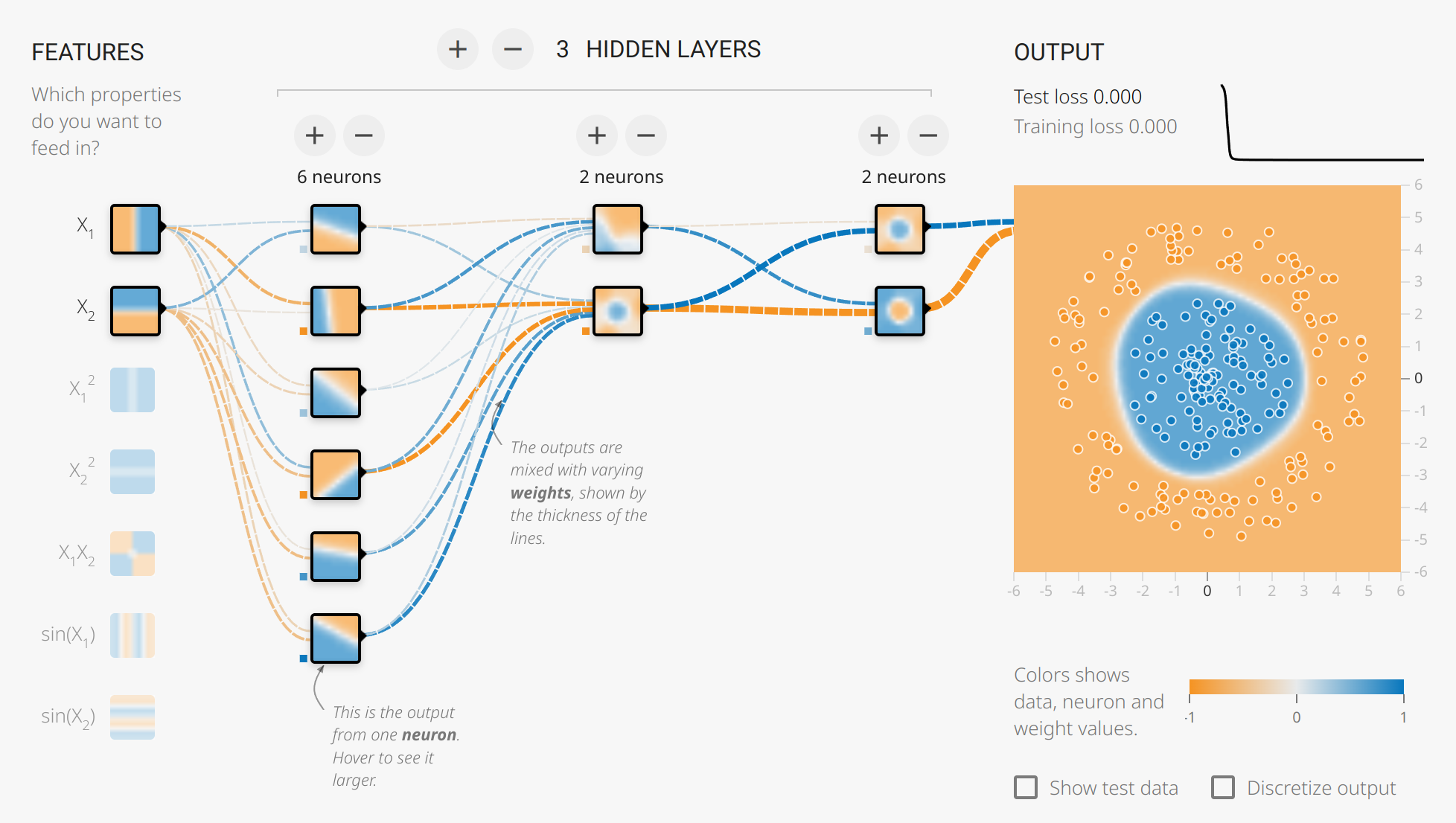
Classification of a circular data using four layers.

Activation Functions

Activation functions decide whether a neuron should be activated or not by calculating the weighted sum and further adding bias to it. They are differentiable operators for transforming input signals to outputs, while most of them add nonlinearity. Because activation functions are fundamental to deep learning, let’s briefly survey some common ones.

ReLU Function

The most popular choice, due to both simplicity of implementation and its good performance on a variety of predictive tasks, is the rectified linear unit (ReLU). ReLU provides a very simple nonlinear transformation. Given an element $x$, the function is defined as the maximum of that element and $0$:

Informally, the ReLU function retains only positive elements and discards all negative elements by setting the corresponding activations to 0. To gain some intuition, we can plot the function. As you can see, the activation function is piecewise linear.

When the input is negative, the derivative of the ReLU function is 0, and when the input is positive, the derivative of the ReLU function is $1$. Note that the ReLU function is not differentiable when the input takes value precisely equal to 0. In these cases, we default to the left-hand-side derivative and say that the derivative is 0 when the input is 0. We can get away with this because the input may never actually be zero (mathematicians would say that it is nondifferentiable on a set of measure zero). There is an old adage that if subtle boundary conditions matter, we are probably doing (real) mathematics, not engineering. We plot the derivative of the ReLU function below.

Derivative for the ReLU function.

The reason for using ReLU is that its derivatives are particularly well behaved: either they vanish or they just let the argument through. This makes optimization better behaved and it mitigated the well-documented problem of vanishing gradients that plagued previous versions of neural networks (more on this later).

Note that there are many variants to the ReLU function, including the parametrized ReLU (pReLU) function He.Zhang.Ren.ea.2015

This variation adds a linear term to ReLU, so some information still gets through, even when the argument is negative:

Sigmoid Function

The sigmoid function transforms those inputs whose values lie in the domain $`\mathbb{R}$, to outputs that lie on the interval $(0, 1)$. For that reason, the sigmoid is often called a squashing function: it squashes any input in the range (-inf, inf) to some value in the range (0, 1):

In the earliest neural networks, scientists were interested in modeling biological neurons that either fire or do not fire. Thus the pioneers of this field, going all the way back to McCulloch and Pitts, the inventors of the artificial neuron, focused on thresholding units . A thresholding activation takes value 0 when its input is below some threshold and value 1 when the input exceeds the threshold.

When attention shifted to gradient-based learning, the sigmoid function was a natural choice because it is a smooth, differentiable approximation to a thresholding unit. Sigmoids are still widely used as activation functions on the output units when we want to interpret the outputs as probabilities for binary classification problems: you can think of the sigmoid as a special case of the softmax. However, the sigmoid has largely been replaced by the simpler and more easily trainable ReLU for most use in hidden layers. Much of this has to do with the fact that the sigmoid poses challenges for optimization since its gradient vanishes for large positive and negative arguments. This can lead to plateaus that are difficult to escape from. Nonetheless sigmoids are important. In later on recurrent neural networks, we will describe architectures that leverage sigmoid units to control the flow of information across time.

Below, we plot the sigmoid function. Note that when the input is close to 0, the sigmoid function approaches a linear transformation.

Plot for the sigmoid function.

The derivative of the sigmoid function is given by the following equation:

The derivative of the sigmoid function is plotted below. Note that when the input is 0, the derivative of the sigmoid function reaches a maximum of 0.25. As the input diverges from 0 in either direction, the derivative approaches 0.

Gradient for the sigmoid function

Tanh Function

Like the sigmoid function, the tanh (hyperbolic tangent) function also squashes its inputs, transforming them into elements on the interval between $-1$ and $1$:

We plot the tanh function below. Note that as input nears $0$, the tanh function approaches a linear transformation. Although the shape of the function is similar to that of the sigmoid function, the tanh function exhibits point symmetry about the origin of the coordinate system.

Plot for the tanh function

The derivative of the tanh function is:

It is plotted below. As the input nears 0, the derivative of the tanh function approaches a maximum of 1. And as we saw with the sigmoid function, as input moves away from 0 in either direction, the derivative of the tanh function approaches 0.

Plot for the gradient for the tanh.

We could not cover all the list of activation function. But we recommend the interted reader for

Activations function in neural networks

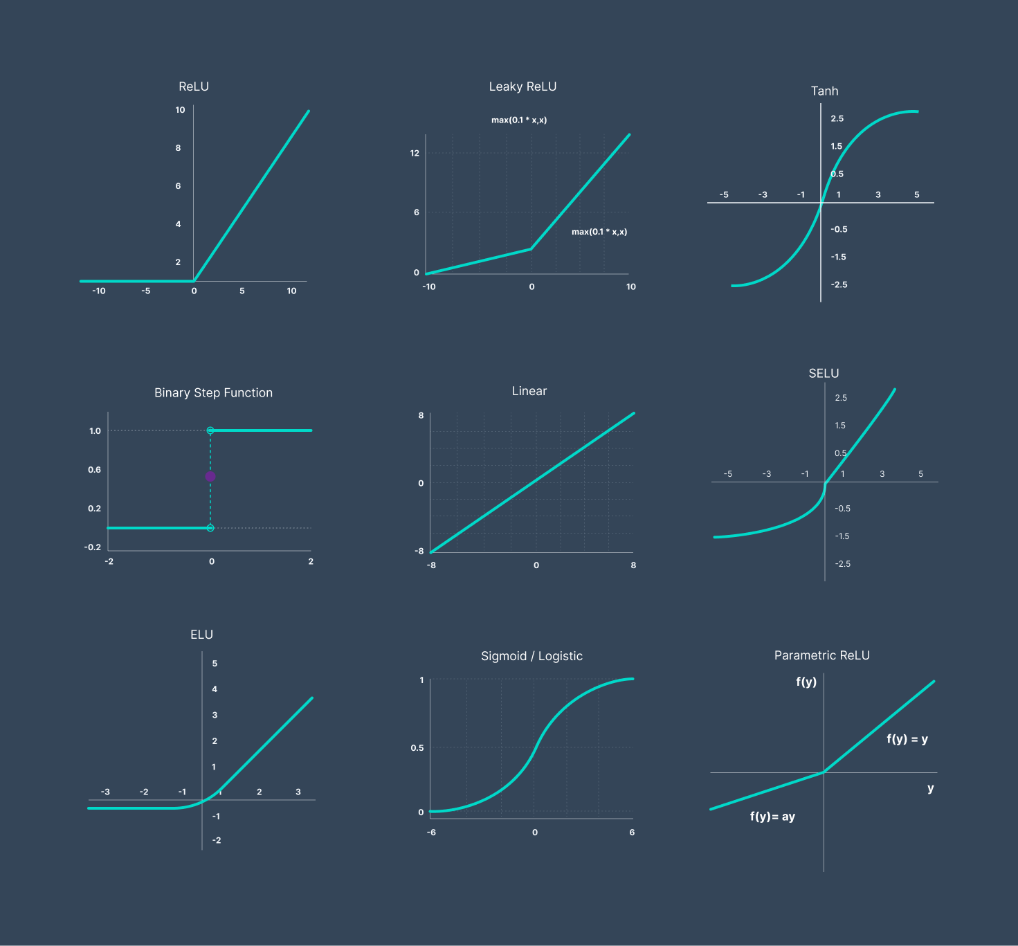
List of activation functions in Deep learning

Forward Propagation, Backward Propagation, and Computational Graphs

In this section, we take a deep dive into the details of backward propagation (more commonly called backpropagation). To convey some insight for both the techniques and their implementations, we rely on some basic mathematics and computational graphs. To start, we focus our exposition on a one-hidden-layer MLP with weight decay ($\ell_2$) regularization, to be described in subsequent chapters).

Forward Propagation

Forward propagation (or forward pass) refers to the calculation and storage of intermediate variables (including outputs) for a neural network in order from the input layer to the output layer. We now work step-by-step through the mechanics of a neural network with one hidden layer. This may seem tedious but in the eternal words of funk virtuoso James Brown, you must pay the cost to be the boss.

For the sake of simplicity, let’s assume that the input example is $\mathbf{x}\in \mathbb{R}^d$ and that our hidden layer does not include a bias term. Here the intermediate variable is:

where $\mathbf{W}^{(1)} \in \mathbb{R}^{h \times d}$ is the weight parameter of the hidden layer. After running the intermediate variable $\mathbf{z}\in \mathbb{R}^h$ through the activation function $\phi$ we obtain our hidden activation vector of length $h$:

The hidden layer output $\mathbf{h}$ is also an intermediate variable. Assuming that the parameters of the output layer possess only a weight of $\mathbf{W}^{(2)} \in \mathbb{R}^{q \times h}$, we can obtain an output layer variable with a vector of length $q$:

Assuming that the loss function is $l$ and the example label is $y$, we can then calculate the loss term for a single data example,

As we will see the definition of g$\ell_2$ regularization to be introduced later, given the hyperparameter g$\lambda$, the regularization term is

where the Frobenius norm of the matrix is simply the $\ell_2$ norm applied after flattening the matrix into a vector. Finally, the models regularized loss on a given data example is:

We refer to $J$ as the objective function in the following discussion.

Computational Graph of Forward Propagation

Plotting computational graphs helps us visualize the dependencies of operators and variables within the calculation. The following figure contains the graph associated with the simple network described above, where squares denote variables and circles denote operators. The lower-left corner signifies the input and the upper-right corner is the output. Notice that the directions of the arrows (which illustrate data flow) are primarily rightward and upward.

Computational graph of forward propagation.

Backpropagation

Now we come to the intersting part. How can we compute the gradient.

A first very bad idea, is to do it by hand.

Given the complexity for Deep learning models, this quickly becomes unfeasible.

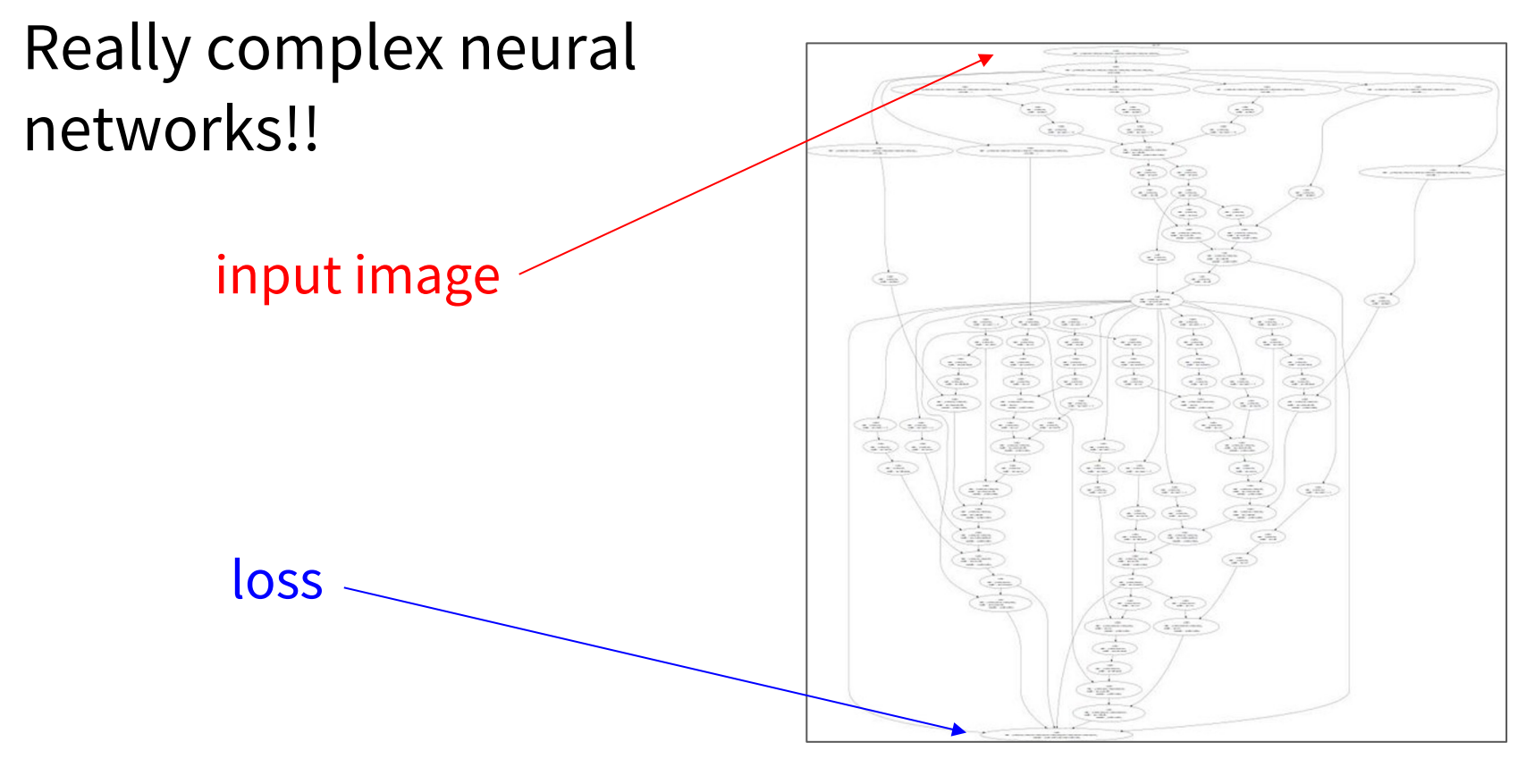
Complexity of deep learning models and how it becomes impossible to compute the gradient of the loss by hand.

Backpropagation refers to the method of calculating the gradient of neural network parameters. In short, the method traverses the network in reverse order, from the output to the input layer, according to the chain rule from calculus. The algorithm stores any intermediate variables (partial derivatives) required while calculating the gradient with respect to some parameters. Assume that we have functions $\mathsf{Y}=f(\mathsf{X})$ and $\mathsf{Z}=g(\mathsf{Y})$ in which the input and the output $\mathsf{X}, \mathsf{Y}, \mathsf{Z}$ are tensors of arbitrary shapes. By using the chain rule, we can compute the derivative of $\mathsf{Z}$ with respect to $\mathsf{X}$ via

Here we use the $\textrm{prod}$ operator to multiply its arguments after the necessary operations, such as transposition and swapping input positions, have been carried out. For vectors, this is straightforward: it is simply matrix matrix multiplication. For higher dimensional tensors, we use the appropriate counterpart. The operator $\textrm{prod}$ hides all the notational overhead.

Recall that the parameters of the simple network with one hidden layer, whose computational graph are $\mathbf{W}^{(1)}$ and $\mathbf{W}^{(2)}$. The objective of backpropagation is to calculate the gradients $\partial J/\partial \mathbf{W}^{(1)}$ and $\partial J/\partial \mathbf{W}^{(2)}$. To accomplish this, we apply the chain rule and calculate, in turn, the gradient of each intermediate variable and parameter. The order of calculations are reversed relative to those performed in forward propagation, since we need to start with the outcome of the computational graph and work our way towards the parameters. The first step is to calculate the gradients of the objective function $J=L+s$ with respect to the loss term $L$ and the regularization term $s$:

Next, we compute the gradient of the objective function with respect to variable of the output layer $\mathbf{o}$ according to the chain rule:

Next, we calculate the gradients of the regularization term with respect to both parameters:

Now we are able to calculate the gradient $\partial J/\partial \mathbf{W}^{(2)} \in \mathbb{R}^{q \times h}$ of the model parameters closest to the output layer. Using the chain rule yields:

To obtain the gradient with respect to $\mathbf{W}^{(1)}$ we need to continue backpropagation along the output layer to the hidden layer. The gradient with respect to the hidden layer output $\partial J/\partial \mathbf{h} \in \mathbb{R}^h$ is given by

Since the activation function $\phi$ applies elementwise, calculating the gradient $\partial J/\partial \mathbf{z} \in \mathbb{R}^h$ of the intermediate variable $\mathbf{z}$ requires that we use the elementwise multiplication operator, which we denote by \odot:

Finally, we can obtain the gradient $\partial J/\partial \mathbf{W}^{(1)} \in \mathbb{R}^{h \times d}$ of the model parameters closest to the input layer. According to the chain rule, we get

Generalization in Deep Learning

We can recall that fitting the training data was only an intermediate goal. Our real quest all along was to discover general patterns on the basis of which we can make accurate predictions even on new examples drawn from the same underlying population. Machine learning researchers are consumers of optimization algorithms. Sometimes, we must even develop new optimization algorithms. But at the end of the day, optimization is merely a means to an end. At its core, machine learning is a statistical discipline and we wish to optimize training loss only insofar as some statistical principle (known or unknown) leads the resulting models to generalize beyond the training set.

On the bright side, it turns out that deep neural networks trained by stochastic gradient descent generalize remarkably well across myriad prediction problems, spanning

• computer vision
• Natural language processing.
• Time series data.
• Recommender systems.
• Electronic health records.
• Protein folding;
• Value function approximation in video games and board games.

Both the theory and practice of deep learning are rapidly evolving, with theorists adopting new strategies to explain what’s going on, even as practitioners continue to innovate at a blistering pace, building arsenals of heuristics for training deep networks and a body of intuitions and folk knowledge that provide guidance for deciding which techniques to apply in which situations.

Revisiting Overfitting and Regularization

According to the No Free Launc theorem, any learning algorithm generalizes better on data with certain distributions, and worse with other distributions. Thus, given a finite training set, a model relies on certain assumptions: to achieve human-level performance it may be useful to identify inductive biases that reflect how humans think about the world. Such inductive biases show preferences for solutions with certain properties. For example, a deep MLP has an inductive bias towards building up a complicated function by the composition of simpler functions.

With machine learning models encoding inductive biases, our approach to training them typically consists of two phases:

1. Fit the training data;
2. Estimate the generalization error (the true error on the underlying population) by evaluating the model on holdout data.

The difference between our fit on the training data and our fit on the test data is called the generalization gap and when this is large, we say that our models overfit to the training data. In extreme cases of overfitting, we might exactly fit the training data, even when the test error remains significant. And in the classical view, the interpretation is that our models are too complex, requiring that we either shrink the number of features, the number of nonzero parameters learned, or the size of the parameters as quantified.

Classical Regularization Methods for Deep Networks

We described several classical regularization techniques for constraining the complexity of our models. In the chapter of optimisation, we introduced a method called weight decay, which consists of adding a regularization term to the loss function in order to penalize large values of the weights. Depending on which weight norm is penalized this technique is known either as ridge regularization (for $\ell_2$ penalty) or lasso regularization (for an $\ell_1$ penalty). In the classical analysis of these regularizers, they are considered as sufficiently restrictive on the values that the weights can take to prevent the model from fitting arbitrary labels.

In deep learning implementations, weight decay remains a popular tool. However, researchers have noted that typical strengths of $\ell_2$ regularization are insufficient to prevent the networks from interpolating the data and thus the benefits if interpreted as regularization might only make sense in combination with the early stopping criterion. Absent early stopping, it is possible that just like the number of layers or number of nodes (in deep learning) or the distance metric (in 1-nearest neighbor), these methods may lead to better generalization not because they meaningfully constrain the power of the neural network but rather because they somehow encode inductive biases that are better compatible with the patterns found in datasets of interests. Thus, classical regularizers remain popular in deep learning implementations, even if the theoretical rationale for their efficacy may be radically different.

Dropout

Let’s think briefly about what we expect from a good predictive model. We want it to peform well on unseen data. Classical generalization theory suggests that to close the gap between train and test performance, we should aim for a simple model. Simplicity can come in the form of a small number of dimensions. Bishop formalized this idea when he proved that training with **input noise is equivalent to Tikhonov regularization. This work drew a clear mathematical connection between the requirement that a function be smooth (and thus simple), and the requirement that it be resilient to perturbations in the input.

After that Srivastava.Hinton.Krizhevsky.ea.2014 developed a clever idea for how to apply Bishop’s idea to the internal layers of a network, too. Their idea, called dropout, involves injecting noise while computing each internal layer during forward propagation, and it has become a standard technique for training neural networks. The method is called dropout because we literally drop out some neurons during training. Throughout training, on each iteration, standard dropout consists of zeroing out some fraction of the nodes in each layer before calculating the subsequent layer.

The key challenge is how to inject this noise. One idea is to inject it in an unbiased manner so that the expected value of each layers while fixing the others equals the value it would have taken absent noise. In Bishop’s work, he added Gaussian noise to the inputs to a linear model. At each training iteration, he added noise sampled from a distribution with mean zero $\epsilon \sim \mathcal{N}(0,\sigma^2)$ to the input $\mathbf{x}$, yielding a perturbed point $\mathbf{x} = \mathbf{x} + \epsilon$. In expectation, $E[\mathbf{x}’] = \mathbf{x}$.

In standard dropout regularization, one zeros out some fraction of the nodes in each layer and then debiases each layer by normalizing by the fraction of nodes that were retained (not dropped out). In other words, with dropout probability $p$, each intermediate activation $h$ is replaced by a random variable $h’$ as follows:

By design, the expectation remains unchanged, i.e., $E[h’] = h$.

Dropout in Practice

Recall the MLP with a hidden layer and five hidden units from the figure of the MLP. When we apply dropout to a hidden layer, zeroing out each hidden unit with probability $p$, the result can be viewed as a network containing only a subset of the original neurons. In the following figure, $h_2$ and $h_5$ are removed. Consequently, the calculation of the outputs no longer depends on $h_2$ or $h_5$ and their respective gradient also vanishes when performing backpropagation. In this way, the calculation of the output layer cannot be overly dependent on any one element of $h_1, \ldots, h_5$.

MLP before and after dropout.

Typically, we disable dropout at test time. Given a trained model and a new example, we do not drop out any nodes and thus do not need to normalize. However, there are some exceptions: some researchers use dropout at test time as a heuristic for estimating the uncertainty of neural network predictions: if the predictions agree across many different dropout outputs, then we might say that the network is more confident.

So in summary, beyond controlling the number of dimensions and the size of the weight vector, dropout is yet another tool for avoiding overfitting. Often tools are used jointly. Note that dropout is used only during training: it replaces an activation $h$ with a random variable with expected value $h$.