The problem of Image classification

Introduction

• Motivation. In this section we will introduce the Image Classification problem, which is the task of assigning an input image one label from a fixed set of categories. This is one of the core problems in Computer Vision that, despite its simplicity, has a large variety of practical applications. Moreover, as we will see later in the course, many other seemingly distinct Computer Vision tasks (such as object detection, segmentation) can be reduced to image classification.

• Example. For example, in the image below an image classification model takes a single image and assigns probabilities to 4 labels, {cat, dog, hat, mug}. As shown in the image, keep in mind that to a computer an image is represented as one large 3-dimensional array of numbers. In this example, the cat image is 248 pixels wide, 400 pixels tall, and has three color channels Red,Green,Blue (or RGB for short). Therefore, the image consists of 248 x 400 x 3 numbers, or a total of 297,600 numbers. Each number is an integer that ranges from 0 (black) to 255 (white). Our task is to turn this quarter of a million numbers into a single label, such as “cat”.

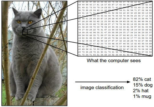
The task in Image Classification is to predict a single label (or a distribution over labels as shown here to indicate our confidence) for a given image. Images are 3-dimensional arrays of integers from 0 to 255, of size Width x Height x 3. The 3 represents the three color channels Red, Green, Blue.

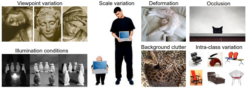
• Challenges. Since this task of recognizing a visual concept (e.g. cat) is relatively trivial for a human to perform, it is worth considering the challenges involved from the perspective of a Computer Vision algorithm. As we present (an inexhaustive) list of challenges below, keep in mind the raw representation of images as a 3-D array of brightness values:
• Viewpoint variation. A single instance of an object can be oriented in many ways with respect to the camera. Scale variation. Visual classes often exhibit variation in their size (size in the real world, not only in terms of their extent in the image).
• Deformation. Many objects of interest are not rigid bodies and can be deformed in extreme ways.
• Occlusion. The objects of interest can be occluded. Sometimes only a small portion of an object (as little as few pixels) could be visible.
• Illumination conditions. The effects of illumination are drastic on the pixel level.
• Background clutter. The objects of interest may blend into their environment, making them hard to identify. Intra-class variation.

The classes of interest can often be relatively broad, such as chair. There are many different types of these objects, each with their own appearance. A good image classification model must be invariant to the cross product of all these variations, while simultaneously retaining sensitivity to the inter-class variations.

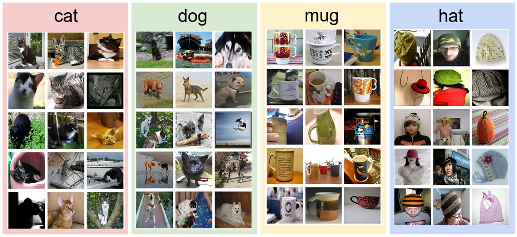
Data-driven approach. How might we go about writing an algorithm that can classify images into distinct categories? Unlike writing an algorithm for, for example, sorting a list of numbers, it is not obvious how one might write an algorithm for identifying cats in images. Therefore, instead of trying to specify what every one of the categories of interest look like directly in code, the approach that we will take is not unlike one you would take with a child: we’re going to provide the computer with many examples of each class and then develop learning algorithms that look at these examples and learn about the visual appearance of each class. This approach is referred to as a data-driven approach, since it relies on first accumulating a training dataset of labeled images. Here is an example of what such a dataset might look like:

CIFAR 10

One popular toy image classification dataset is the CIFAR-10 dataset.

• This dataset consists of 60,000 tiny images that are 32 pixels high and wide.
• Each image is labeled with one of 10 classes (for example “airplane, automobile, bird, etc”).
• These 60,000 images are partitioned into a training set of 50,000 images and a test set of 10,000 images.
• In the image below you can see 10 random example images from each one of the 10 classes:

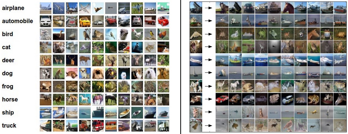
Example images from the CIFAR-10 dataset. Right: first column shows a few test images and next to each we show the top 10 nearest neighbors in the training set according to pixel-wise difference.

Let’s consider some notations which follows the standard in Machine Learning:

• Training data :

• $n$ is the dimentionality of the input data.
• $k$ is the number of classes.
• $m$ is the number of points in the training set.

So for the CIFAR we have:

• $n = 32\times 32 = 1024$
• $m = 50000$
• $k = 10$.

Can you think of an hypothesis function for this problem?

Nearest Neighbor Classifier

As our first approach, we will develop what we call a Nearest Neighbor Classifier. This classifier has nothing to do with Deep Learning and it is very rarely used in practice, but it will allow us to get an idea about the basic approach to an image classification problem.

The nearest neighbor classifier will take a test image, compare it to every single one of the training images, and predict the label of the closest training image. In the image above and on the right you can see an example result of such a procedure for 10 example test images. Notice that in only about 3 out of 10 examples an image of the same class is retrieved, while in the other 7 examples this is not the case. For example, in the 8th row the nearest training image to the horse head is a red car, presumably due to the strong black background. As a result, this image of a horse would in this case be mislabeled as a car.

You may have noticed that we left unspecified the details of exactly how we compare two images, which in this case are just two blocks of 32 x 32 x 3. One of the simplest possibilities is to compare the images pixel by pixel and add up all the differences. In other words, given two images and representing them as vectors $I1$,$I2$ , a reasonable choice for comparing them might be the \(L1\) distance:

Where the sum is taken over the pixels.

Here is an example of such difference:

An example of using pixel-wise differences to compare two images with L1 distance (for one color channel in this example). Two images are subtracted elementwise and then all differences are added up to a single number. If two images are identical the result will be zero. But if the images are very different the result will be large.

In your first assignement you will have to implement this classifier with the following structure

import numpy as np

class NearestNeighbor(object):
  def __init__(self):
    pass

  def train(self, X, y):
    """ X is N x D where each row is an example.
    Y is 1-dimension of size N """

    # the nearest neighbor classifier simply remembers
    #all the training data
    self.Xtr = X
    self.ytr = y

  def predict(self, X):
    """ X is N x D where each row is an example we wish
    to predict label for """
    num_test = X.shape[0]
    # lets make sure that the output type matches the input type
    Ypred = np.zeros(num_test, dtype = self.ytr.dtype)
    pass

The choice of distance. There are many other ways of computing distances between vectors. Another common choice could be to instead use the $L_2$ distance, which has the geometric interpretation of computing the euclidean distance between two vectors. The distance takes the form:

L1 vs. L2: It is interesting to consider differences between the two metrics. In particular, the L2 distance is much more unforgiving than the L1 distance when it comes to differences between two vectors. That is, the L2 distance prefers many medium disagreements to one big one. L1 and L2 distances (or equivalently the L1/L2 norms of the differences between a pair of images) are the most commonly used special cases of a p-norm

You may have noticed that it is strange to only use the label of the nearest image when we wish to make a prediction. Indeed, it is almost always the case that one can do better by using what’s called a k-Nearest Neighbor Classifier. The idea is very simple: instead of finding the single closest image in the training set, we will find the top k closest images, and have them vote on the label of the test image. In particular, when k = 1, we recover the Nearest Neighbor classifier. Intuitively, higher values of k have a smoothing effect that makes the classifier more resistant to outliers:

An example of the difference between Nearest Neighbor and a 5-Nearest Neighbor classifier, using 2-dimensional points and 3 classes (red, blue, green). The colored regions show the decision boundaries induced by the classifier with an L2 distance. The white regions show points that are ambiguously classified (i.e. class votes are tied for at least two classes). Notice that in the case of a NN classifier, outlier datapoints (e.g. green point in the middle of a cloud of blue points) create small islands of likely incorrect predictions, while the 5-NN classifier smooths over these irregularities, likely leading to better generalization on the test data (not shown). Also note that the gray regions in the 5-NN image are caused by ties in the votes among the nearest neighbors (e.g. 2 neighbors are red, next two neighbors are blue, last neighbor is green).

Multiclass Support Vector Machine loss

As a second example we will develop a commonly used loss called the Multiclass Support Vector Machine (SVM) loss. The SVM loss is set up so that the SVM “wants” the correct class for each image to a have a score higher than the incorrect classes by some fixed margin $\Delta$ . Notice that it’s sometimes helpful to anthropomorphise the loss functions as we did above: The SVM “wants” a certain outcome in the sense that the outcome would yield a lower loss (which is good).

Let’s now get more precise. Recall that for the i-th example we are given the pixels of image $x_i$ and the label $y_i$ that specifies the index of the correct class. The score function takes the pixels and computes the vector $f(x_i,W)$ of class scores, which we will abbreviate to $s$ (short for scores). For example, the score for the j-th class is the j-th element: $s_j=f(xi,W)_j$. The Multiclass SVM loss for the i-th example is then formalized as follows:

Example: Lets unpack this with an example to see how it works. Suppose that we have three classes that receive the scores s=$[13,−7,11]$, and that the first class is the true class (i.e. $y_i=0$). Also assume that $\Delta$ (a hyperparameter we will go into more detail about soon) is 10. The expression above sums over all incorrect classes ($j\neq y_i$) ), so we get two terms:

You can see that the first term gives zero since $[-7 - 13 + 10]$ gives a negative number, which is then thresholded to zero with the $max(0,−)$ function. We get zero loss for this pair because the correct class score (13) was greater than the incorrect class score (-7) by at least the margin 10. In fact the difference was 20, which is much greater than 10 but the SVM only cares that the difference is at least 10; Any additional difference above the margin is clamped at zero with the max operation. The second term computes $[11 - 13 + 10]$ which gives 8. That is, even though the correct class had a higher score than the incorrect class (13 > 11), it was not greater by the desired margin of 10. The difference was only 2, which is why the loss comes out to 8 (i.e. how much higher the difference would have to be to meet the margin). In summary, the SVM loss function wants the score of the correct class $y_i$ to be larger than the incorrect class scores by at least by $\Delta$ (delta). If this is not the case, we will accumulate loss.

Note that in this particular module we are working with linear score functions $(f(x_i;W)=Wx_i )$, so we can also rewrite the loss function in this equivalent form:

\(L_i = \sum_{j \neq y_i} \max(0, W_j^Tx_i - W_{y_i}^Tx_i + \Delta)\) where $w_j$ is the j-th row of $W$ reshaped as a column. However, this will not necessarily be the case once we start to consider more complex forms of the score function $f$.

A last piece of terminology we’ll mention before we finish with this section is that the threshold at zero $max(0,−)$ function is often called the hinge loss. You’ll sometimes hear about people instead using the squared hinge loss SVM (or L2-SVM), which uses the form $max(0,−)^2$ that penalizes violated margins more strongly (quadratically instead of linearly). The unsquared version is more standard, but in some datasets the squared hinge loss can work better. This can be determined during cross-validation.

The loss function quantifies our unhappiness with predictions on the training set

The Multiclass Support Vector Machine "wants" the score of the correct class to be higher than all other scores by at least a margin of delta. If any class has a score inside the red region (or higher), then there will be accumulated loss. Otherwise the loss will be zero. Our objective will be to find the weights that will simultaneously satisfy this constraint for all examples in the training data and give a total loss that is as low as possible.

Regularisation

There is one bug with the loss function we presented above. Suppose that we have a dataset and a set of parameters $W$ that correctly classify every example (i.e. all scores are so that all the margins are met, and $L_i=0\;\;\forall i$). The issue is that this set of $W$ is not necessarily unique: there might be many similar $W$ that correctly classify the examples. One easy way to see this is that if some parameters $W$ correctly classify all examples (so loss is zero for each example), then any multiple of these parameters $\lambda W$ where $\lambda>1$ will also give zero loss because this transformation uniformly stretches all score magnitudes and hence also their absolute differences. For example, if the difference in scores between a correct class and a nearest incorrect class was $15$, then multiplying all elements of $W$ by $2$ would make the new difference $30$.

In other words, we wish to encode some preference for a certain set of weights $\mathbf{W}$ over others to remove this ambiguity. We can do so by extending the loss function with a regularization penalty $R(W)$ . The most common regularization penalty is the squared $L_2$-norm that discourages large weights through an elementwise quadratic penalty over all parameters:

In the expression above, we are summing up all the squared elements of W . Notice that the regularization function is not a function of the data, it is only based on the weights. Including the regularization penalty completes the full Multiclass Support Vector Machine loss, which is made up of two components: the data loss (which is the average loss $L_i$ over all examples) and the regularization loss. That is, the full Multiclass SVM loss becomes:

or in the full form:

Where $N$ is the number of training examples and $\lambda$ is an hyperparameter to balance between the data loss and the regularization term. There is no simple way of setting this hyperparameter and it is usually determined by cross-validation.

Softmax classifier

It turns out that the SVM is one of two commonly seen classifiers. The other popular choice is the Softmax classifier, which has a different loss function. If you’ve heard of the binary Logistic Regression classifier before, the Softmax classifier is its generalization to multiple classes. Unlike the SVM which treats the outputs $f(x_i,W)$ as (uncalibrated and possibly difficult to interpret) scores for each class, the Softmax classifier gives a slightly more intuitive output (normalized class probabilities) and also has a probabilistic interpretation that we will describe shortly. In the Softmax classifier, the function mapping f$(x_i;W)=Wx_i$ stays unchanged, but we now interpret these scores as the unnormalized log probabilities for each class and replace the hinge loss with a cross-entropy loss that has the form:

where we are using the notation $f_j$ to mean the j-th element of the vector of class scores $f$. As before, the full loss for the dataset is the mean of $L_i$ over all training examples together with a regularization term $R(W)$. The function $f_j(z)=\dfrac{e^{z_j}}{\sum_k e^{z_k}}$ is called the softmax function: It takes a vector of arbitrary real-valued scores (in z) and squashes it to a vector of values between zero and one that sum to one. The full cross-entropy loss that involves the softmax function might look scary if you’re seeing it for the first time but it is relatively easy to motivate.

Probabilistic interpretation. Looking at the expression, we see that

can be interpreted as the (normalized) probability assigned to the correct label $y_i$ given the image $x_i$ and parameterized by $W$. To see this, remember that the Softmax classifier interprets the scores inside the output vector $f$ as the unnormalized log probabilities. Exponentiating these quantities therefore gives the (unnormalized) probabilities, and the division performs the normalization so that the probabilities sum to one. In the probabilistic interpretation, we are therefore minimizing the negative log likelihood of the correct class, which can be interpreted as performing Maximum Likelihood Estimation (MLE). A nice feature of this view is that we can now also interpret the regularization term $R(W)$ in the full loss function as coming from a Gaussian prior over the weight matrix $W$ , where instead of MLE we are performing the Maximum a posteriori (MAP) estimation. We mention these interpretations to help your intuitions, but the full details of this derivation are beyond the scope of this class.

Practical issues: Numeric stability. When you’re writing code for computing the Softmax function in practice, the intermediate terms $e^{f_{y_i}}$ and $\sum_j e^{f_j}$ may be very large due to the exponentials. Dividing large numbers can be numerically unstable, so it is important to use a normalization trick. Notice that if we multiply the top and bottom of the fraction by a constant $C$ and push it into the sum, we get the following (mathematically equivalent) expression

We are free to choose the value of $C$. This will not change any of the results, but we can use this value to improve the numerical stability of the computation. A common choice for $C$ is to set $\log C=−\max_jf_j$. This simply states that we should shift the values inside the vector f so that the highest value is zero. In code:

f = np.array([123, 456, 789]) # example with 3 classes and each having large scores
p = np.exp(f) / np.sum(np.exp(f)) # Bad: Numeric problem, potential blowup

# instead: first shift the values of f so that the highest number is 0:
f -= np.max(f) # f becomes [-666, -333, 0]
p = np.exp(f) / np.sum(np.exp(f)) # safe to do, gives the correct answer

SVM vs. Softmax

A picture might help clarify the distinction between the Softmax and SVM classifiers:

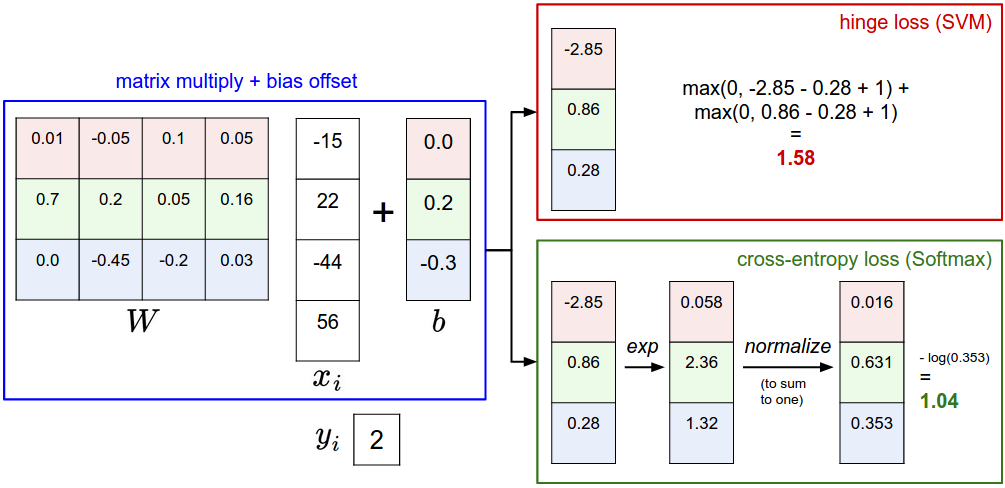
Example of the difference between the SVM and Softmax classifiers for one datapoint. In both cases we compute the same score vector f (e.g. by matrix multiplication in this section). The difference is in the interpretation of the scores in f: The SVM interprets these as class scores and its loss function encourages the correct class (class 2, in blue) to have a score higher by a margin than the other class scores. The Softmax classifier instead interprets the scores as (unnormalized) log probabilities for each class and then encourages the (normalized) log probability of the correct class to be high (equivalently the negative of it to be low). The final loss for this example is 1.58 for the SVM and 1.04 (note this is 1.04 using the natural logarithm, not base 2 or base 10) for the Softmax classifier, but note that these numbers are not comparable; They are only meaningful in relation to loss computed within the same classifier and with the same data.

In your first homework you will implement both classifiers and check difference in action.