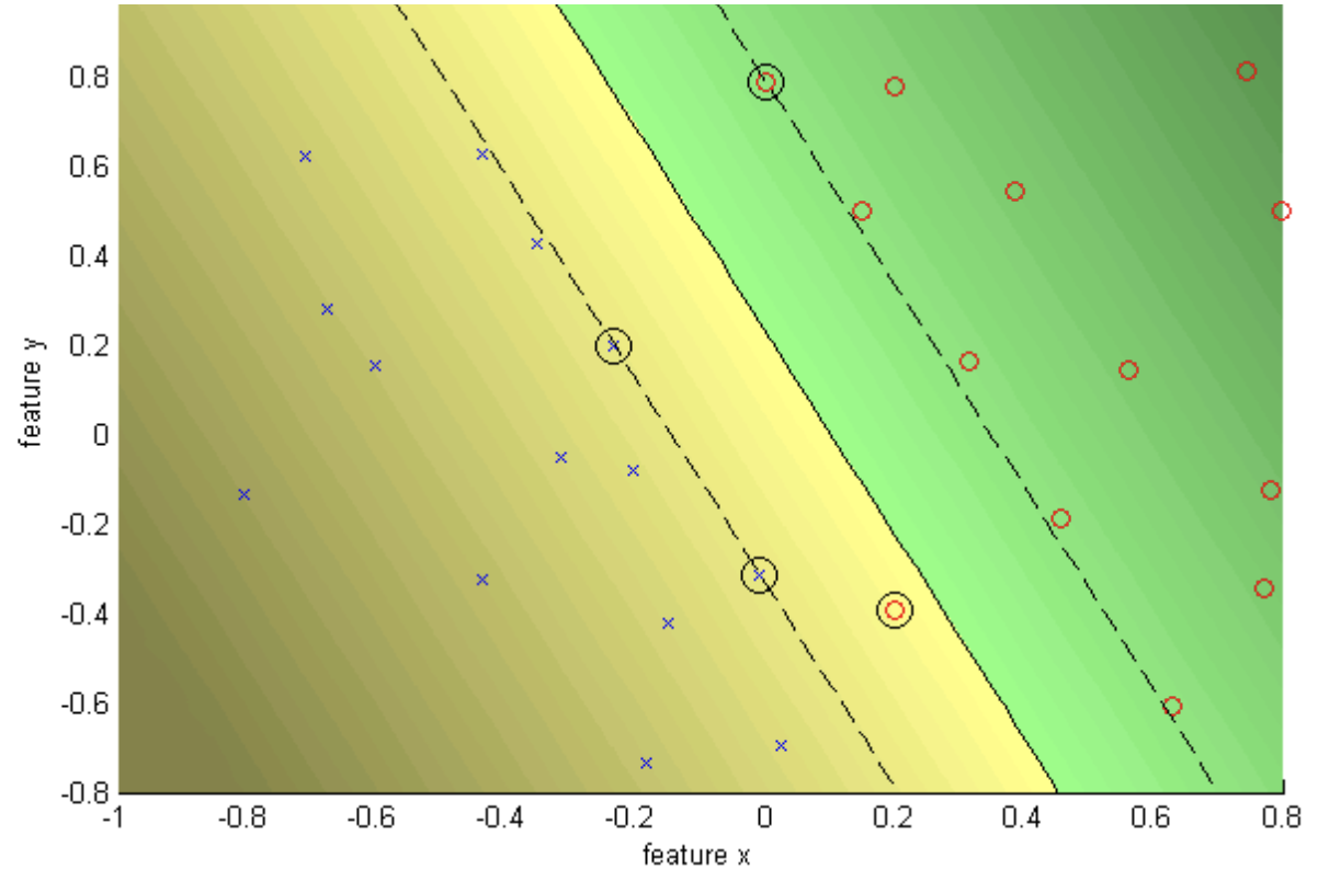
Classification with Support Vector Machine

Binary Classification

In binary classification, we aim to classify data points into one of two distinct classes, often represented by labels $+1$ and $-1$. This problem is fundamental in machine learning and has applications across many fields, such as:

• Medical diagnosis
• Spam detection
• Image recognition.

The goal is to learn a function ( f(x) ) that accurately distinguishes between the two classes based on training data.

Given training data $(x_i, y_i)$ for $i = 1, \ldots, N $, where each $ x_i \in \mathbb{R}^d $ represents a data point in a $d$-dimensional space, and $ y_i \in {-1, 1} $ is the corresponding class label, our task is to construct a classifier $f(x)$ such that:

This requirement can be summarized as:

which means that for a correct classification, the product $ y_i f(x_i) $ should be positive. If $ f(x_i) $ has the same sign as $ y_i$, the classification is correct; otherwise, it is incorrect. The objective of binary classification is to find $ f(x) $ that maximizes correct classifications on unseen data, effectively generalizing the patterns learned from the training data.

Lineary Separability

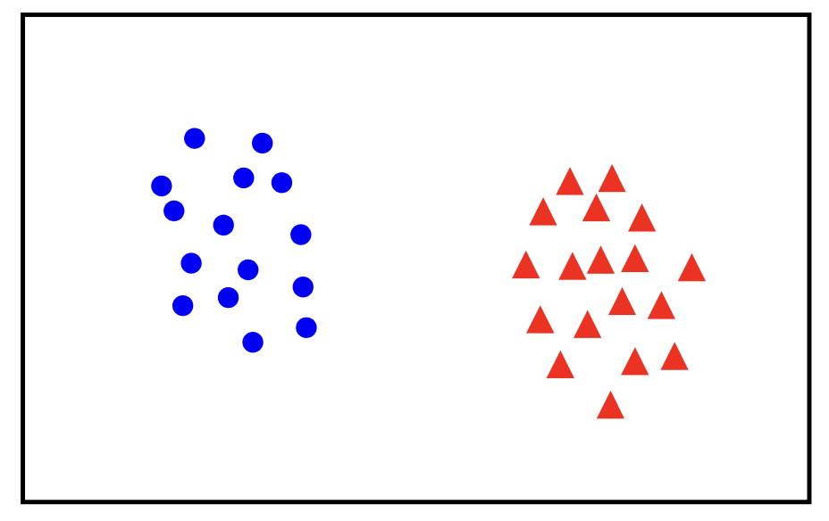
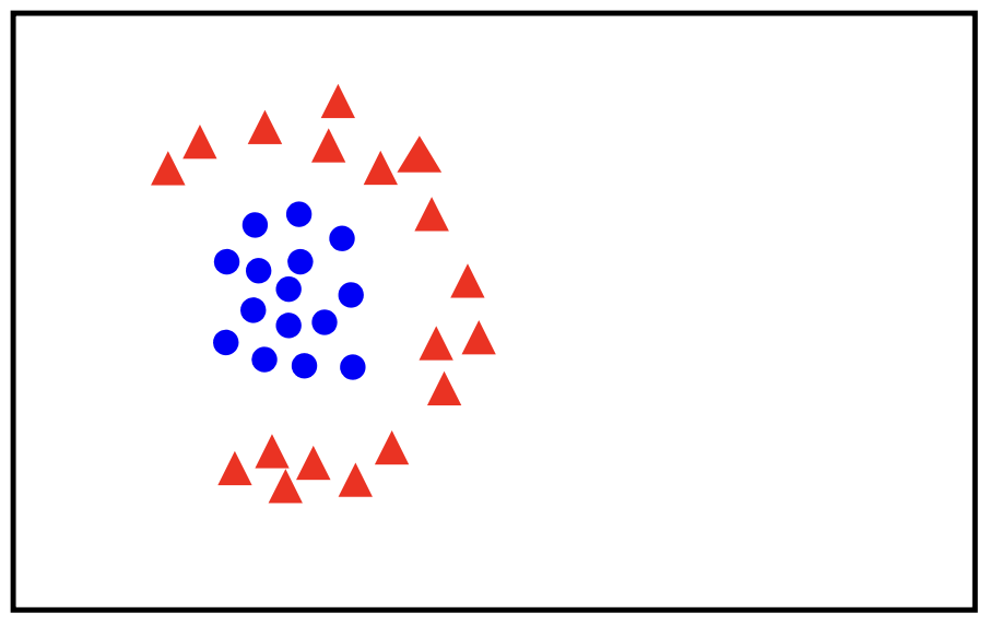
In a linearly separable problem, we assume that the data can be separated into two classes using a straight line (in two dimensions), a plane (in three dimensions), or, more generally, a hyperplane in higher dimensions. This means that there exists a linear decision boundary, defined by a linear function $ f(x) = w \cdot x + b $, that perfectly divides the data points into two groups, each belonging to one of the classes.

Linear models, like those used in linearly separable classifications, are computationally efficient and interpretable. They provide a straightforward approach to classifying data, especially when working with high-dimensional feature spaces where complex decision boundaries may not be necessary. However, linear models have limitations: they struggle with data that is not linearly separable, meaning that classes overlap in a way that cannot be split by a single hyperplane. In these cases, more flexible or nonlinear models are often needed to capture complex relationships within the data.

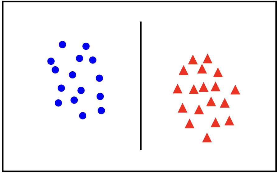
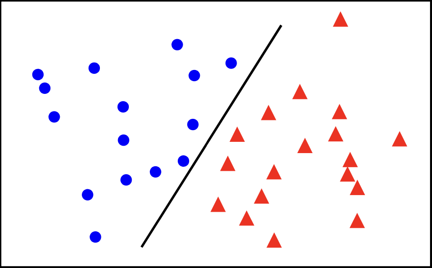
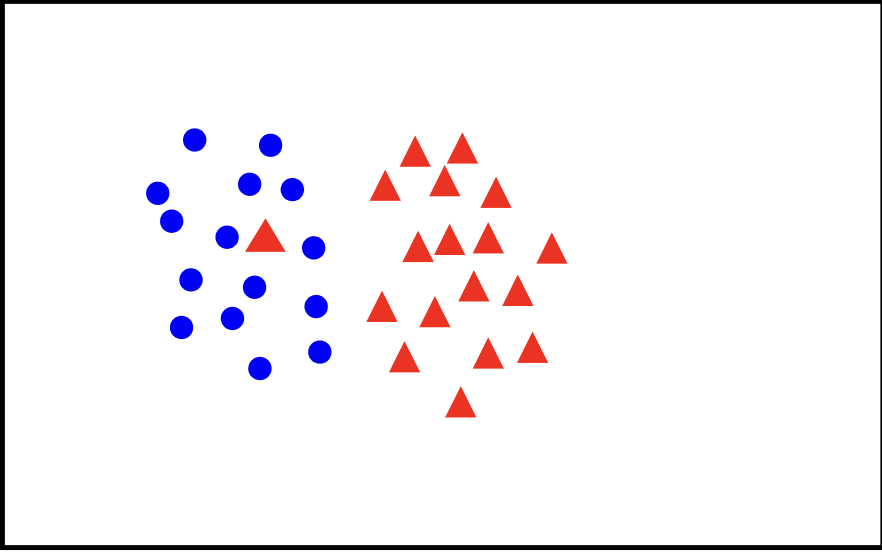
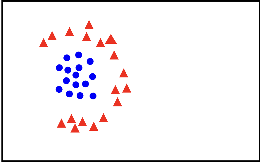
Linear Classifier

A linear classifier aims to separate data into distinct classes using a linear boundary, which, in two-dimensional space, is represented as a line and, in higher dimensions, as a hyperplane.

The classifier seeks to find this optimal line or hyperplane such that the separation between classes is maximized, ideally placing all data points from one class on one side and those from the other class on the opposite side.

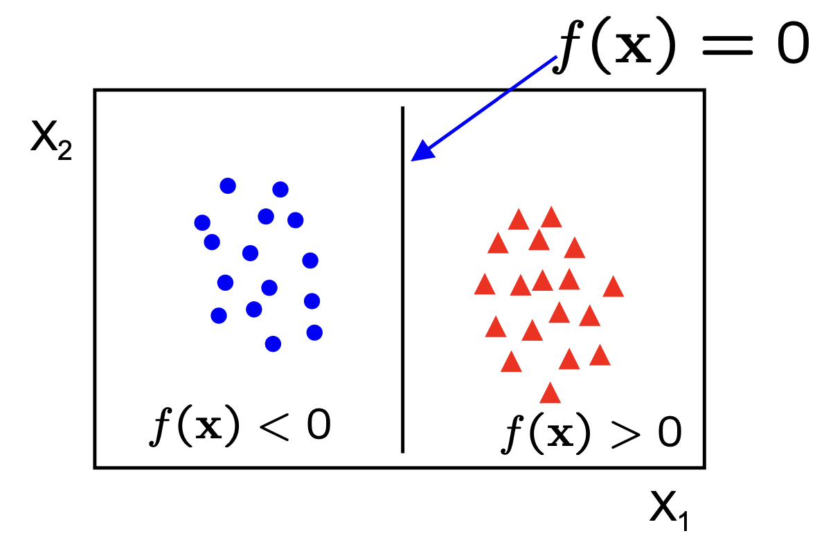
Mathematically, the decision boundary is defined by the equation

where $ w $ is the weight vector normal to the hyperplane, $x$ represents the input features, and $ b $ is the bias term. The classifier then makes predictions based on which side of the hyperplane a given data point lies.

• $w$ is the normal to the line and $b$ is the bias.
• $w$ is also known as the weight vector.

In 2D the discriminant is a plane and in $nD$ the discriminant is an hyperplane.

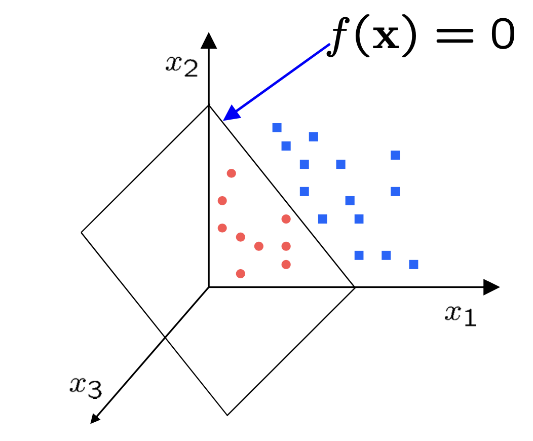
Perceptron Classifier

The perceptron classifier is a fundamental algorithm used for binary classification tasks. It is a type of linear classifier that attempts to find a hyperplane to separate data points from two different classes. The basic perceptron algorithm works iteratively.

We write the classifier as

where

1. Initialize $w = 0$.
2. Cycle through the dataset $(x_i,y_i)$
   • if $x_i$ is misclassified then

\(w \leftarrow w + \alpha \text{sign}(f(x_i))x_i\)

1. Until all the data is correctly classified.

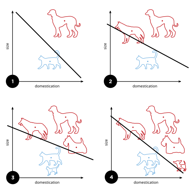
• If the data is linearly separable, then the algorithm will converge.
• Convergence can be slow
• Separating line close to training data.
• We would prefer a larger margin for generalization.

So this bring the question what would be the best $W$ or the best margin for generalization.

Let’s consider the following data?

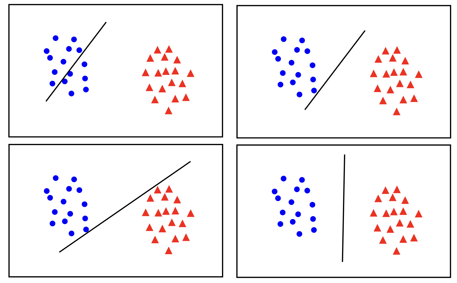
The best classifier has the biggest margin which makes it sable under perturbation.

Support Vector Machine (SVM)

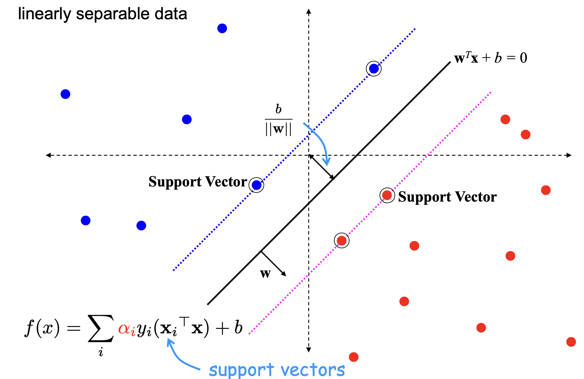
Keys ideas behind SVM

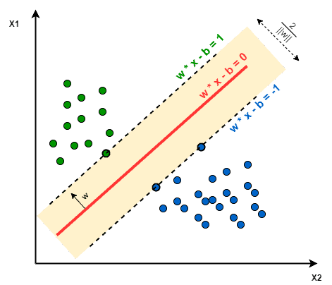
1. Since $w^T\cdot x + b = 0$ and $c(w^T\cdot x + b) = 0$ define the same plane, we have the freedom to choose the normalization of $w$

2. Choose normalization such that
   • $w^T\cdot x_+ + b = +1$
   • $w^T\cdots x_- +b =−1$ for the positive and negative support vectors re-spectively
3. Then the margin is given by

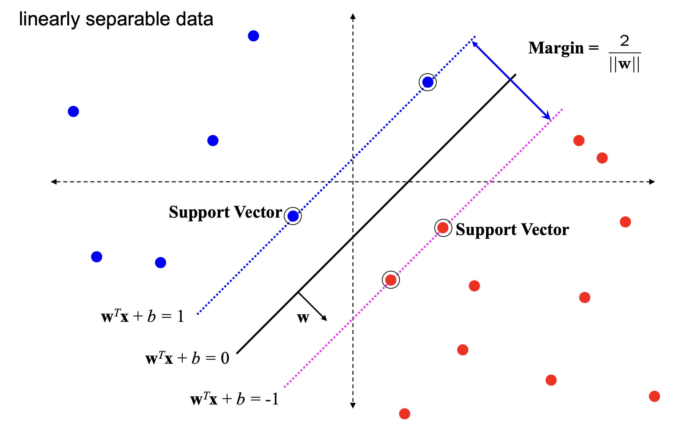
Hence Getting the best line on SVM is equivalent to an optimisization problem which is given by the optimization problem for maximizing the margin between the closest data points $\mathbf{x}+$ and $\mathbf{x}-$ can be formulated as follows:

subject to the constraint:

This formulation ensures that the margin $\frac{2}{|\mathbf{w}|}$ is maximized, given the constraints that data points.

The quadratic optimization problem for the Support Vector Machine (SVM) can be formulated as:

subject to the constraints:

This is a quadratic optimization problem subject to linear constraints and there is a unique minimum

Slack Variables

Slack variables are introduced in the SVM optimization problem to handle cases where the data is not perfectly linearly separable. They allow some data points to be misclassified or lie within the margin, enabling a more flexible decision boundary. The importance of slack variables lies in their ability to create a better trade-off between maximizing the margin and minimizing classification errors. By allowing some points to be incorrectly classified or closer to the hyperplane, the SVM can achieve a wider margin, which often leads to better generalization on new, unseen data. The next figure will illustrate how allowing a few misclassified points can lead to a more robust and effective decision boundary.

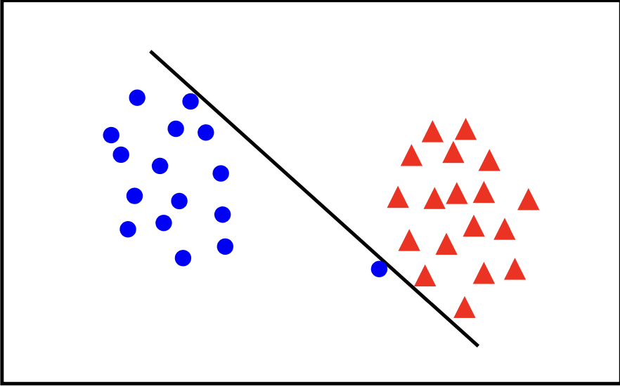
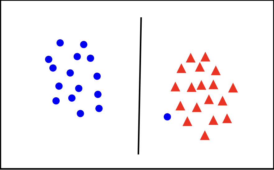
In general there is a tradoff between the margin and the number of mistakes on the training data.

The key idea is to introduce a new hyper-parameter called $\xi$ that should decide if the point is misclassified or just a margin violation.

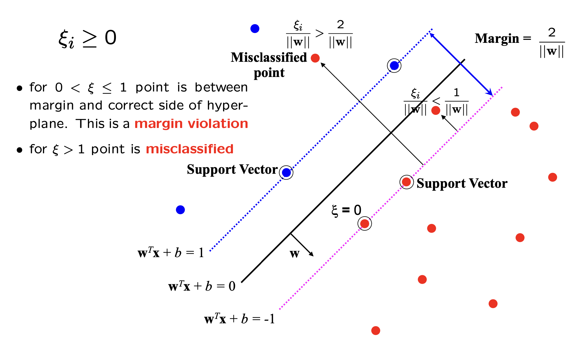
the optimization problems becomes:

subject to:

We remark that

• Every Constraint can be satisfied if $\xi$ is large enough.
• $C$ is called the regularisation parameter.
  • Small $C$ allows constraints to be easily ignored. $\rightarrow$ Large margin.
  • Large $C$ makes constraintes hard to ignore. $\rightarrow$ narrow margin.
  • $C = \infty$ enforces all the constraints. $\rightarrow$ hard margin.

Let’s consider the following example:

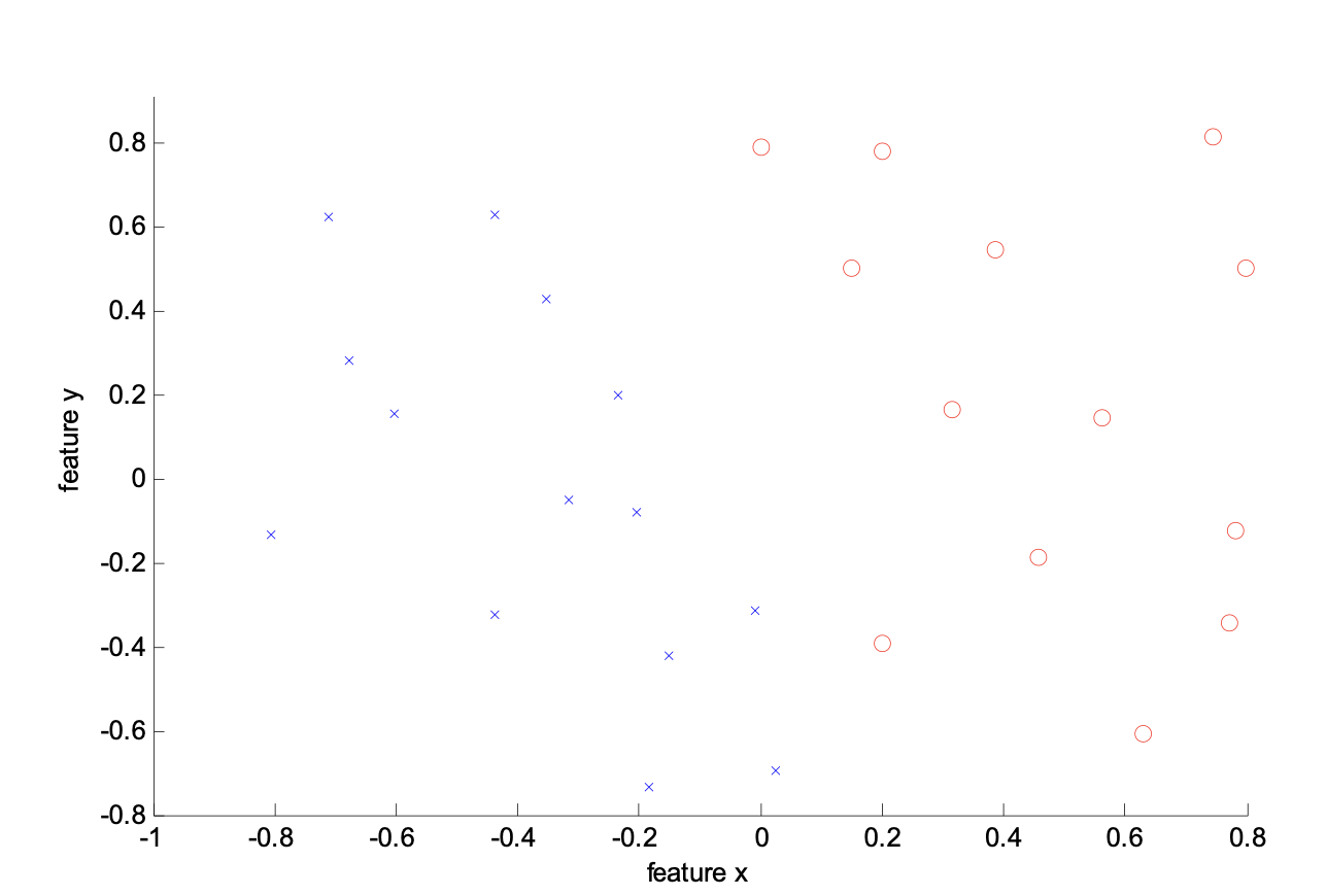
The data looks linearly separable but the margin is very narrow. Here is the separation for the data with $C = \infty$.

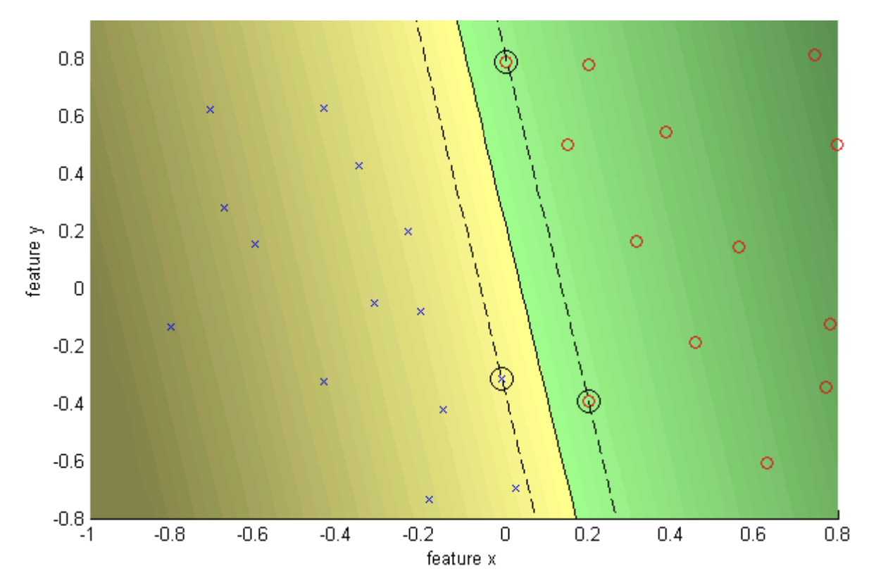
And here is a better separation with a soft margin using $C = 10$.