Data Similarity

Similarity and Dissimilarity Measures
Data similarity and dissimilarity measures are foundational to numerous data analysis techniques, including clustering, classification, and anomaly detection. In essence, measuring similarity (or dissimilarity) between data points allows us to group, classify, and compare data, which is critical for machine learning, data mining, and even everyday applications like recommendation systems or search engines.
-
Similarity: This refers to how alike two data points are. Similar items are grouped together in tasks like clustering or nearest neighbor searches. Here are some properties for similarity measure.
- A numerical measure of a how alike data objects are.
- Is higher when objects are more alike.
- Often falls in the range $[0,1]$.
-
Dissimilarity (Distance): This is the opposite how different two data points are. Many machine learning algorithms use distance metrics to quantify this dissimilarity.
- Numerical measure of how different objects are.
- Lower when objects are more alike.
- Minimum dissimilarity is $0$.
- Upper limit may varies.
The right measure of similarity depends on the type of data and the task at hand. For example, Euclidean distance is suitable for continuous numeric data, whereas Cosine similarity is preferred for textual data or vectors representing angles.
By understanding how different similarity and distance measures work, we can improve the performance of models and make better data-driven decisions.
simple Attributes
The following table shows the similarity and dissimilarity between two objects, $x$ and $y$, with respect to a single, simple attribute
| Attribute Type | Similarity | Dissimilarity |
|---|---|---|
| Nominal |
\( s(x, y) = \begin{cases} 1 & \text{if } x = y \\ 0 & \text{if } x \neq y \end{cases} \) |
\( d(x, y) = \begin{cases} 0 & \text{if } x = y \\ 1 & \text{if } x \neq y \end{cases} \) |
| Ordinal |
\( s(x, y) = 1 - \frac{|r(x) - r(y)|}{n-1} \) |
\( d(x, y) = \frac{|r(x) - r(y)|}{n-1} \) |
| Interval/Ratio |
\( s= -1, s = \dfrac{1}{1+d}, s = e^{-d}\) |
\( d(x, y) = \vert x - y\vert \) |
Euclidian Distance
Euclidean distance is one of the most widely used distance measures, particularly for continuous numerical data. It is the “ordinary” straight-line distance between two points in Euclidean space. This metric is based on the Pythagorean theorem, and it calculates the distance between two points as the length of the shortest path between them.
In an $n$-dimensional space, the Euclidean distance between two points $x = (x_1, x_2, \dots, x_n)$ and $ y = (y_1, y_2, \dots, y_n)$ is calculated as follows:
\[d(x, y) = \sqrt{(x_1 - y_1)^2 + (x_2 - y_2)^2 + \dots + (x_n - y_n)^2}\]This formula represents the sum of squared differences between corresponding coordinates of the two points, followed by the square root of the result. Euclidean distance is commonly used in clustering, classification, and other machine learning algorithms.
let’s consider the example where we will calculate the Euclidean distances between four points in a 2-dimensional space:
- $ P_1 = (0, 2) $
- $ P_2 = (2, 0) $
- $ P_3 = (3, 1) $
- $ P_4 = (5, 1) $
Each of these points represents coordinates in a 2D space, and we will compute the Euclidean distance between every pair of points to form a distance matrix.
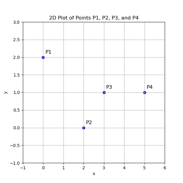
Here is a summary for the euclidien distances
| P1 | P2 | P3 | P4 | |
|---|---|---|---|---|
| P1 | 0.000 | 2.828 | 3.162 | 5.099 |
| P2 | 2.828 | 0.000 | 1.414 | 3.162 |
| P3 | 3.162 | 1.414 | 0.000 | 2.000 |
| P4 | 5.099 | 3.162 | 2.000 | 0.000 |
Minkowski Distance
Minkowski distance is a generalized metric used to measure the distance between two points in a normed vector space. It is a generalization of both the Euclidean and Manhattan distances, and it allows for varying levels of flexibility through the parameter ( r ). When ( r = 1 ), it becomes the Manhattan distance; when ( r = 2 ), it reduces to the Euclidean distance. For larger values of ( r ), the distance gives more weight to larger differences between coordinates. As ( r ) approaches infinity, the Minkowski distance becomes the Chebyshev distance, which only considers the maximum difference between dimensions.
The formula for Minkowski distance between two points $ x = (x_1, x_2, \dots, x_n) $ and $ y = (y_1, y_2, \dots, y_n)$ is:
\[d(x, y) = \left( \sum_{i=1}^{n} |x_i - y_i|^r \right)^{\frac{1}{r}}\]For more information, you can refer to Minkowski Distance on Wikipedia.

Special Cases of Minkowski Distance
Here are the special cases of the Minkowski distance when ( r ) takes specific values:
-
$ r = 1$ : This is known as the Manhattan distance or L1 norm. It is calculated as the sum of the absolute differences between the coordinates of the points.
\[d(x, y) = \sum_{i=1}^{n} |x_i - y_i|\] -
$ r = 2 $ : This is the Euclidean distance or L2 norm, where the distance is the square root of the sum of the squared differences between the coordinates.
\[d(x, y) = \sqrt{\sum_{i=1}^{n} (x_i - y_i)^2}\] -
$ r = \infty $ : This is known as the Chebyshev distance or L∞ norm. It considers only the maximum absolute difference between the coordinates.
\[d(x, y) = \max(|x_1 - y_1|, |x_2 - y_2|, \dots, |x_n - y_n|)\]
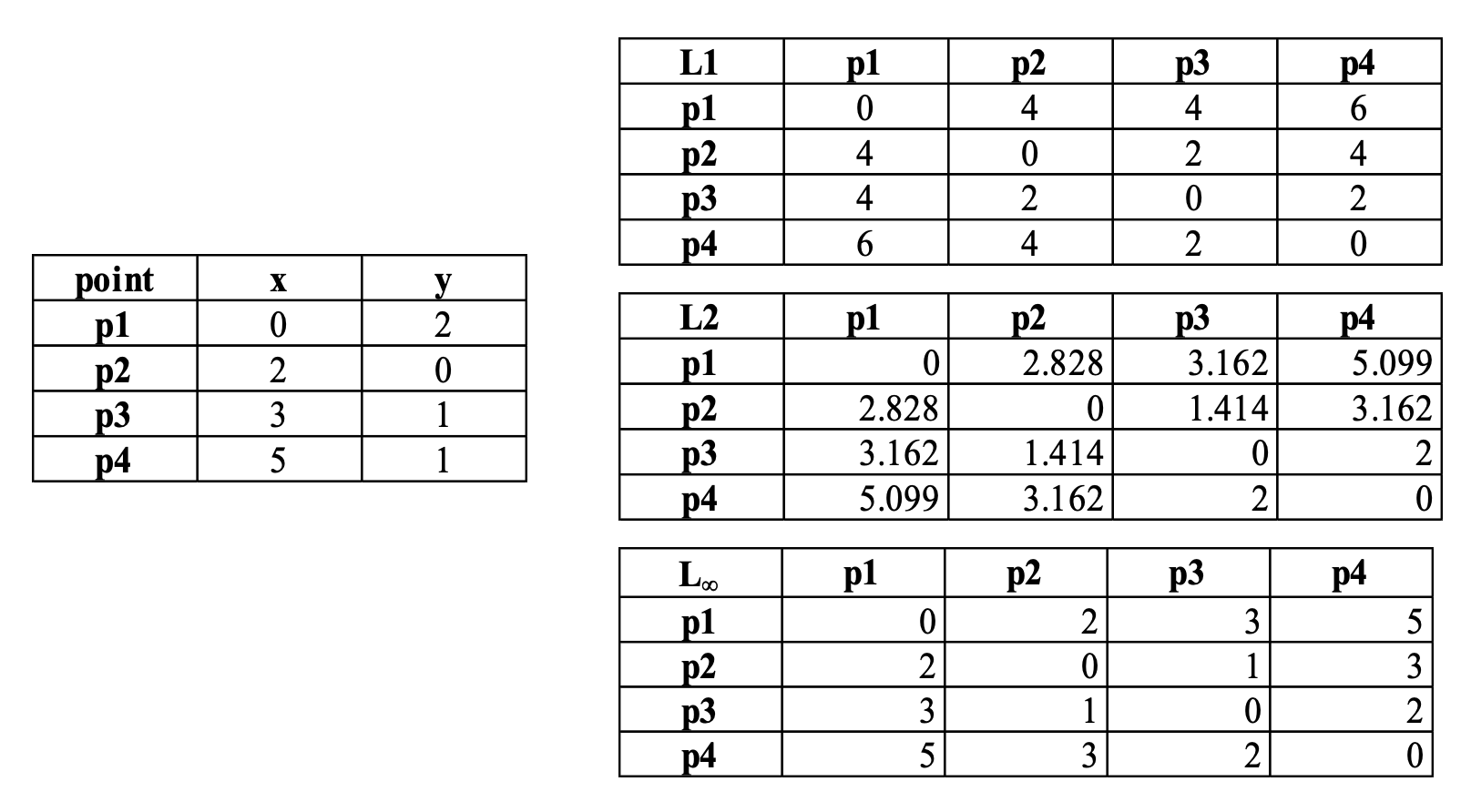
Comparison between the three classical distances (L1, L2, L_infiny) on the proposed points).
Mahalanobis Distance
Mahalanobis distance is a measure of the distance between a point and a distribution. Unlike Euclidean distance, which only considers the direct spatial distance between points, Mahalanobis distance takes into account the correlations of the dataset by using the covariance matrix. It is particularly useful in identifying outliers in multivariate data and measuring similarity in data with different scales.
The formula for Mahalanobis distance between a vector $x$ and a vector $y$ is:
\[d(x, y) = \sqrt{(x - y)^T \Sigma^{-1} (x - y)}\]Where:
- $ (x - y) $ is the difference vector between the two points.
- $ \Sigma^{-1} $ is the inverse of the covariance matrix of the data.
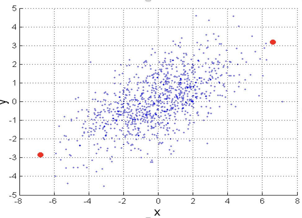
Let’s consider the following example:
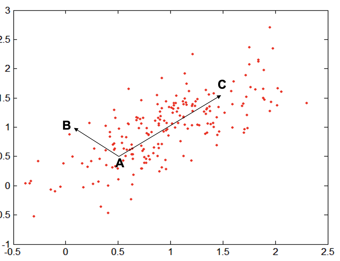
where:
- $A = (0.5, 0.5)$ , $B = (0,1)$ and $C =(1.5,1.5)$.
- The covariance of the dataset is
We will obtain that:
- $D(A,B) = 5$
- $D(A,C) = 4$
Common properties
In distance-based algorithms, it is important to recognize that all classical distance measures, including Euclidean distance, Manhattan distance, Minkowski distance, and Mahalanobis distance, adhere to three fundamental properties:
- Non-negativity:
- All distances are non-negative. The distance between any two points $ x $ and $ y $, represented as $ d(x, y) $, is always greater than or equal to zero.
The distance is zero only when the points are identical: ( d(x, y) = 0 ) if and only if ( x = y ).
- Symmetry:
- The distance between two points is the same regardless of the direction of measurement. In other words, the distance from $ x $ to $ y $ is the same as the distance from $ y $ to $ x $.
- Triangle Inequality:
- For any three points $ x $, $ y $, and $ z $, the distance from $x $ to $ y $ is always less than or equal to the sum of the distances from $ x $ to $ z $ and from $ z $ to $ y $. This property ensures that the shortest distance between two points is a direct line.
These properties ensure that the concept of “distance” behaves intuitively and consistently across different metrics, making them suitable for clustering, classification, and anomaly detection tasks.
Binary Vectors
When working with binary vectors (where each element takes a value of 0 or 1), specific distance and similarity measures are often employed to capture the relationships between these vectors. Two common methods are Simple Matching Coefficient (SMC) and Jaccard Coefficient
Simple Matching Coefficient (SMC)
The Simple Matching Coefficient measures the similarity between two binary vectors by considering both matches of 1s (presence) and 0s (absence). It calculates the proportion of elements that are the same in both vectors, whether they are 1s or 0s.
Given two binary vectors $ A = (a_1, a_2, …, a_n) $ and $ B = (b_1, b_2, …, b_n) $, the Simple Matching Coefficient is defined as:
\[SMC(A, B) = \frac{M_{00} + M_{11}}{M_{00} + M_{01} + M_{10} + M_{11}}\]Where:
- $ M_{11} $ is the number of attributes where both $ A$ and $ B$ have a value of 1.
- $ M_{00}$ is the number of attributes where both $A $ and $ B $ have a value of 0.
- $ M_{01}$ is the number of attributes where $A $ has a 0 and $ B $ has a 1.
- $ M_{10}$ is the number of attributes where $ A$ has a 1 and $ B $ has a 0.
This measure takes into account both matches and mismatches, making it a symmetric similarity measure.
Jaccard Coefficient
The Jaccard Coefficient (or Jaccard Similarity) focuses only on the presence of attributes, ignoring the matches of 0s. It is defined as the size of the intersection divided by the size of the union of two sets, and it is used to measure the similarity between two binary vectors in terms of their shared positive (1) elements.
The Jaccard Coefficient for binary vectors ( A ) and ( B ) is given by:
\[J(A, B) = \frac{M_{11}}{M_{01} + M_{10} + M_{11}}\]Where:
- $ M_{11} $ is the number of attributes where both $ A $ and $ B $ have a value of 1.
- $ M_{01} $ and $ M_{10} $ are the number of attributes where the values of $A $ and $B$ differ.
The Jaccard Coefficient gives more weight to positive matches (1s), making it more suitable for tasks where the presence of attributes (or positive matches) is more meaningful than their absence.
Key Differences:
- SMC considers both matches (1s and 0s), while Jaccard focuses only on the matches of 1s.
- SMC is a symmetric similarity measure, whereas Jaccard is useful when the presence of attributes (1s) is more significant than their absence (0s).
Both of these measures are widely used in clustering and classification tasks when dealing with binary or categorical data.
Let’s consider the two vectors:
- $x = (1, 0, 0, 0, 0, 0, 0, 0 ,0 ,0)$
- $y = (0, 0, 0, 0, 0, 0, 1, 0, 0, 1) $
We will have:
- $M_{01} = 2$
- $M_{10} = 1$
- $M_{00} = 7$
- $M_{11} = 0$
which will give
\[\text{SMC} = \dfrac{0 + 7 }{ 2 + 1 + 0 + 7} = 0.7\]and
\[J = \dfrac{0 }{ 2 + 1 + 0 + 7} = 0\]Cosine Similarity
Cosine Similarity is a measure of similarity between two non-zero vectors of an inner product space. It calculates the cosine of the angle between the two vectors, which reflects how similar the vectors are in terms of direction (rather than magnitude). Cosine similarity is commonly used in applications like text analysis, recommendation systems, and clustering tasks.
The formula for Cosine Similarity between two vectors $ A $ and $ B$ is:
\[\text{Cosine Similarity}(A, B) = \frac{A \cdot B}{\|A\| \|B\|}\]Where:
- $ A \cdot B $ is the dot product of vectors $ A $ and $ B$.
- $ |A| $and $ |B| $ are the magnitudes (or lengths) of vectors $A $ and $ B $, respectively.
The result ranges from -1 (completely opposite) to 1 (completely similar), with 0 indicating orthogonality, meaning the vectors are independent of each other.
Example: Computing Cosine Similarity
Let’s consider two vectors $ A $ and $ B $ of size 10:
- $ A = [1, 2, 3, 4, 5, 6, 7, 8, 9, 10] $
- $ B = [10, 9, 8, 7, 6, 5, 4, 3, 2, 1] $
To compute the Cosine Similarity between these two vectors, follow these steps:
- Compute the dot product:
- Compute the magnitude of each vector:
- Compute the Cosine Similarity:
- Dot Product: $ A \cdot B = 220 $
- Magnitude of $A $: $ |A| = 19.62 $
- Magnitude of $ B $: $ |B| = 19.62 $
- Cosine Similarity: $ \frac{220}{19.62 \times 19.62} = 0.57 $
Correlation
Correlation is a statistical measure that describes the strength and direction of a linear relationship between two variables. The most commonly used measure is Pearson’s correlation coefficient, which quantifies how two variables move in relation to one another. Below are the key elements needed to compute this coefficient.
Covariance measures how much two variables change together. If the variables tend to increase together, the covariance will be positive; if one tends to increase while the other decreases, the covariance will be negative. Mathematically, the covariance between two variables $ A $ and $ B $ is given by:
\[\text{Cov}(A, B) = \frac{1}{n} \sum_{i=1}^{n} (A_i - \bar{A})(B_i - \bar{B})\]Where:
- $ A_i $ and $ B_i $ are the elements of vectors $ A $ and $ B $, respectively.
- $ \bar{A} $ and $ \bar{B} $ are the means of the vectors $ A $ and $ B $.
- $ n $ is the number of elements in the vectors.
The standard deviation measures the amount of variation or dispersion of a set of values from their mean. The standard deviation of a vector ( A ) is calculated as:
\[\text{SD}(A) = \sqrt{\frac{1}{n} \sum_{i=1}^{n} (A_i - \bar{A})^2}\]Similarly, the standard deviation of vector ( B ) is:
\[\text{SD}(B) = \sqrt{\frac{1}{n} \sum_{i=1}^{n} (B_i - \bar{B})^2}\]
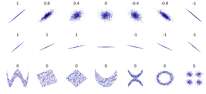
Several sets of (x, y) points, with the Pearson correlation coefficient of x and y for each set. The correlation reflects the noisiness and direction of a linear relationship (top row), but not the slope of that relationship (middle), nor many aspects of nonlinear relationships (bottom). N.B.: the figure in the center has a slope of 0 but in that case, the correlation coefficient is undefined because the variance of Y is zero.
When comparing data points using different distance or similarity measures, it’s important to consider how the data is transformed. Two key transformations that can affect the results of these metrics are scaling and translation:
- Scaling refers to multiplying the entire dataset by a constant factor, which changes the magnitude of the data but not its shape.
- Translation involves shifting all points by adding a constant value, which changes their absolute positions but preserves the relative distances between points.
Different distance and similarity metrics react differently to these transformations:
- Cosine Similarity measures the angle between two vectors and is unaffected by both scaling and translation.
- Euclidean Distance measures the straight-line distance between points and is sensitive to both scaling and translation.
- Correlation measures the linear relationship between two variables and is invariant to scaling but sensitive to translation.
| Metric | Invariant to Scaling | Invariant to Translation |
|---|---|---|
| Cosine Similarity | Yes | No |
| Euclidean Distance | No | No |
| Correlation | Yes | Yes |
let’s consider the example for $x = (1,2,4, 3, 0, 0 ,0)$.
- $ y = (1, 2, 3, 4, 0, 0, 0) $
- $ y $ scaled by 2: $ 2y = (2, 4, 6, 8, 0, 0, 0)$
- $y $ translated by 5: $ y + 5 = (6, 7, 8, 9, 5, 5, 5)$
we will get the following results:
| Metric | y | y scaled by 2 | y translated by 5 |
|---|---|---|---|
| Euclidean Distance | 1.414 | 5.831 | 13.304 |
| Cosine Similarity | 0.967 | 0.967 | 0.826 |
| Correlation | 0.936 | 0.936 | 0.936 |
