Data

Introduction
It’s tempting to jump straight into mining, but first, we need to get the data ready. This involves having a closer look at attributes and data values. Real-world data are typically noisy, enormous in volume (often several gigabytes or more), and may originate from a hodge-podge of heterogenous sources. This chapter is about getting familiar with your data. Knowledge about your data is useful for data preprocessing (see Chapter 3), the first major task of the data mining process. You will want to know the following: What are the types of attributes or fields that make up your data? What kind of values does each attribute have? Which attributes are discrete, and which are continuous-valued? What do the data look like? How are the values distributed? Are there ways we can visualize the data to get a better sense of it all? Can we spot any outliers? Can we measure the similarity of some data objects with respect to others? Gaining such insight into the data will help with the subsequent analysis.
Data Objects and Attributes.
Data sets consist of data objects, which represent entities like customers in a sales database, patients in a medical database, or students in a university database. Data objects are described by attributes and can also be called samples, examples, instances, or data points. In a database, data objects correspond to rows (or data tuples), and attributes correspond to columns. This section defines attributes and explores different attribute types.
| Tid | Refund | Marital Status | Taxable Income | Cheat |
|---|---|---|---|---|
| 1 | Yes | Single | 125K | No |
| 2 | No | Married | 100K | No |
| 3 | No | Single | 70K | No |
| 4 | Yes | Married | 120K | No |
| 5 | No | Divorced | 95K | Yes |
| 6 | No | Married | 60K | No |
| 7 | Yes | Divorced | 220K | No |
| 8 | No | Single | 85K | Yes |
| 9 | No | Married | 75K | No |
| 10 | No | Single | 50K | Yes |
Data Attributes
What is an attribute
An attribute is a data field, representing a characteristic or feature of a data object.
-
The nouns attribute, dimension, feature, and variable are often used interchangeably in the literature. The term dimension is commonly used in data warehousing.
-
Machine learning literature tends to use the term feature,
There are several types of attributes types according to their values.
1. Nominal
Definition:
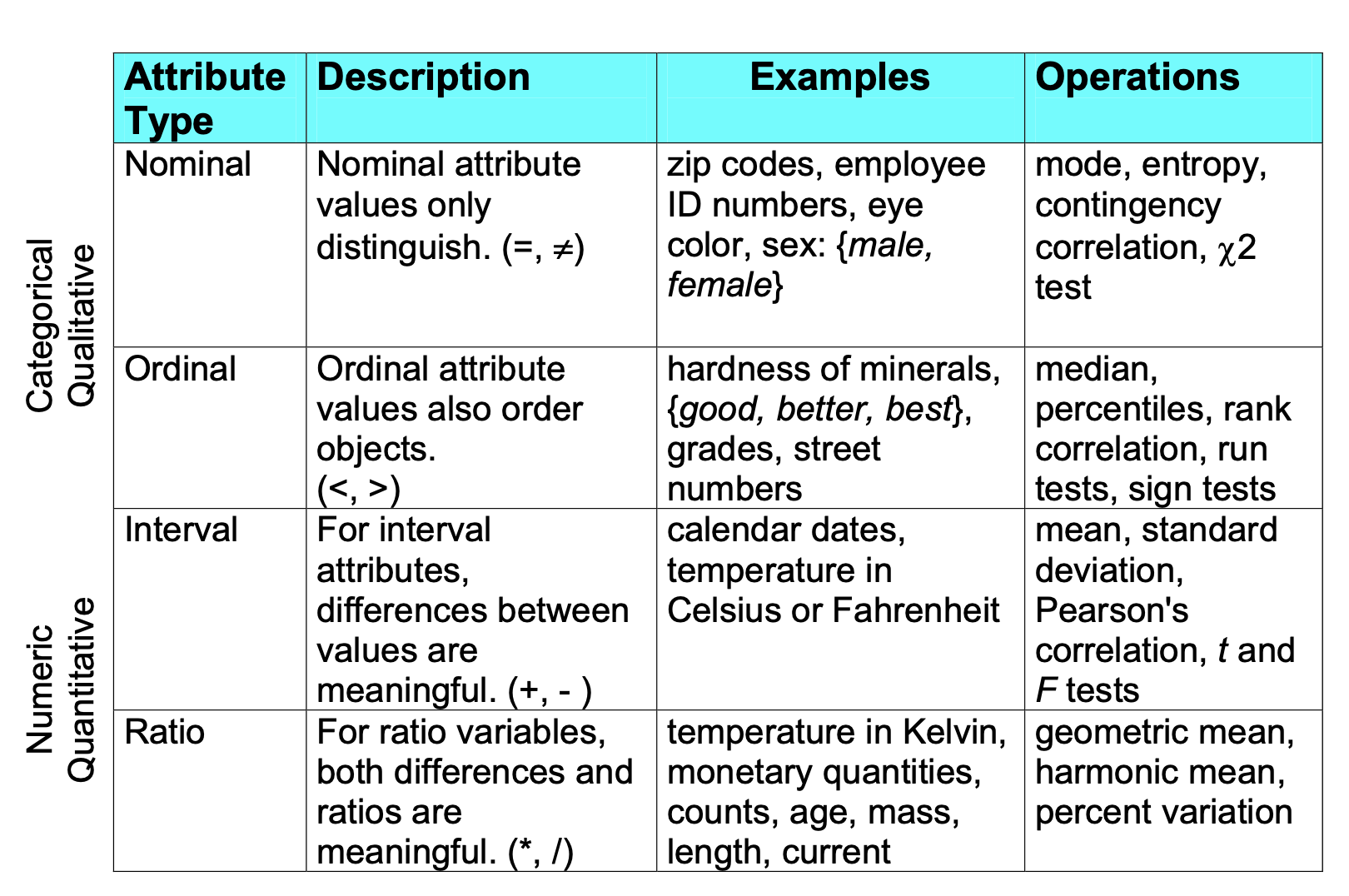
Nominal attributes are qualitative and have no inherent order. They are used to label categories or groups without any numerical significance.
Example:
| ID | Color |
|---|---|
| 1 | Red |
| 2 | Blue |
| 3 | Green |
| 4 | Yellow |
In this example, “Color” is a nominal attribute because the colors do not have an intrinsic order.

2. Binary
Definition:
Binary attributes have two possible states or values, typically represented as 0 and 1, or “Yes” and “No”.
Example:
| ID | Has Pet |
|---|---|
| 1 | Yes |
| 2 | No |
| 3 | Yes |
| 4 | No |
“Has Pet” is a binary attribute with two possible values: “Yes” or “No”.

3. Ordinal
Definition:
Ordinal attributes have a clear, meaningful order, but the differences between the values are not necessarily consistent or measurable.
Example:
| ID | Education Level |
|---|---|
| 1 | High School |
| 2 | Bachelor’s |
| 3 | Master’s |
| 4 | PhD |
In this case, “Education Level” is ordinal because it follows a specific order from lowest to highest education level.

4. Numerical
Numerical attributes have meaningful numerical values, and they can be further classified into two types:
4.1 Interval-scaled
Definition:
Interval-scaled attributes are numerical and have meaningful differences between values, but they do not have a true zero point.
Example:
| ID | Temperature (°C) |
|---|---|
| 1 | 20 |
| 2 | 25 |
| 3 | 30 |
| 4 | 35 |
Here, “Temperature” is an interval-scaled attribute because you can measure the difference between values, but 0°C does not represent the complete absence of temperature.
4.2 Ratio-scaled
Definition:
Ratio-scaled attributes are numerical and have both meaningful differences and a true zero point, which indicates the absence of the attribute.
Example:
| ID | Income ($) |
|---|---|
| 1 | 0 |
| 2 | 5000 |
| 3 | 15000 |
| 4 | 25000 |
“Income” is a ratio-scaled attribute because it has a true zero point (no income) and you can compare values meaningfully using ratios (e.g., $15,000 is three times $5,000).
Difference Between Interval-scaled and Ratio-scaled Attributes:
- Zero Point: The key difference is that ratio-scaled attributes have a true zero point, which means the attribute can be absent (e.g., zero income). Interval-scaled attributes do not have a true zero point (e.g., 0°C does not mean the absence of temperature).
- Ratios: You can meaningfully calculate ratios for ratio-scaled attributes (e.g., one person earning twice as much as another). For interval-scaled attributes, you can only calculate differences, not ratios (e.g., 30°C is not “twice as hot” as 15°C).
This structure should provide a comprehensive explanation of the different types of attributes, complete with examples and a clear explanation of the differences between interval and ratio scales.
We can study the type of an attributes according to the following points:
- Distinctness: Distinctness refers to whether you can determine that two values are different. It’s often represented with symbols like
=or≠. - Order: Order refers to the ability to rank or arrange the values in a meaningful sequence, typically represented by symbols like
<or>. - Differences are meaningful: This property means that you can meaningfully calculate the difference between two values, often represented by
+or-. - Ratios are meaningful: This indicates that you can meaningfully calculate ratios (e.g., one value being twice another), often represented by
*or/.
Table
| Property | Nominal | Binary | Ordinal | Interval-scaled | Ratio-scaled |
|---|---|---|---|---|---|
| Distinctness (eq, neq) | x | x | x | x | x |
| Order ( < > ) | x | x | x | ||
| Differences (+ -) | x | x | |||
| Ratios (* /) | x |
This table summarizes how each data type corresponds to the properties of distinctness, order, differences, and ratios. You can use this to help explain the differences between the types of data attributes.
The categorization of attributes into nominal, ordinal, interval, and ratio scales was introduced by Stanley Smith Stevens, a prominent psychologist and pioneer in the field of experimental psychology. Stevens first described these scales in his 1946 paper "On the theory of scales of measurement," which has become foundational in the fields of psychology, statistics, and data analysis.
Continuous vs Discrete
Discrete data refers to data that can take on only specific, distinct values. These are often countable and have clear boundaries, such as the number of students in a classroom or the outcome of rolling a die. Continuous data, on the other hand, can take any value within a given range, allowing for an infinite number of possible values. This type of data is typically measurable, such as height, temperature, or time. The key distinction is that while discrete data can only assume distinct, separate values, continuous data can vary smoothly across a range. This difference is crucial in determining the appropriate methods for analysis and interpretation.
- Continuous attributes:
- Has only a finite or countably infinite set of values.
- Examples : zip codes, counts, of the set of words in a collection of documents.
- Often represented as an integer variable
- Note: binary attributes are a special case of discrete attributes.
- Continuous attributes:
- Has real numbers as attributes values.
- Examples: temperature, height, or weight.
- Practically: Real values can be represented using a finite number of digits.
Characteristics of Data
- Dimensionality (number of attributes)
- High-dimensional data brings a number of challenges.
- Sparsity
- Only presence counts.
- Resolution
- Patterns depend on the scale.
- Size
- Type of analysis may depend on the size of the data.
Dimensionality refers to the number of attributes or features present in a dataset. High-dimensional data presents unique challenges, including increased computational complexity and the potential for overfitting in models. As the number of dimensions increases, the data space becomes increasingly sparse, making it harder to find meaningful patterns.
Sparsity emphasizes that in high-dimensional datasets, only the presence of certain features may be significant, while the absence of data (zeros or nulls) is often less informative. This means that in many cases, only the non-zero values or active features in the data are considered important.
Resolution is the level of detail in the data. The patterns and trends that can be identified in the data often depend on the scale at which the data is examined. Finer resolution can reveal detailed patterns, while coarser resolution might obscure them.
Size of the data is another critical characteristic, as it can influence the type of analysis that is feasible. Large datasets might require more robust computational resources and more sophisticated analytical techniques, while smaller datasets might limit the statistical power of the analysis.
Types of Data Sets
Data sets can be categorized into different types based on their structure and the nature of the information they contain. Understanding the types of data sets is essential for selecting the appropriate methods of analysis and processing. Below is a classification of data set types that reflects their varied structures and applications
- Record:
- Data Matrix.
- Document Data.
- Transaction Data.
- Graph:
- World Wide Web.
- Molecular Structures.
- Ordered:
- Spatial Data
- Temporal Data.
- Sequential Data.
- Genetic Sequence Data.
Record Data
Record data consists of a collection of records, each of which consists of a fixed set of attributes.
| Tid | Refund | Marital Status | Taxable Income | Cheat |
|---|---|---|---|---|
| 1 | Yes | Single | 125K | No |
| 2 | No | Married | 100K | No |
| 3 | No | Single | 70K | No |
Data Matrix
If data objects have the same fixed set of numeric attributes, then the data objects can be thought of as points in a multi-dimensional space, where each dimension represents a distinct attribute
Such a data set can be represented by an m by n matrix, where there are m rows, one for each object, and n columns, one for each attribute.
| Algebra | Data Mining | Machine Learning | System Admin |
|---|---|---|---|
| 12 | 35 | 78 | 23 |
| 15 | 42 | 81 | 29 |
| 18 | 38 | 75 | 26 |
| 20 | 40 | 80 | 30 |
Document Data
Each document becomes a ‘term’ vector.
- Each term is a component (attribute) of the vector
- The value of each component is the number of times the corresponding term occurs in the document.
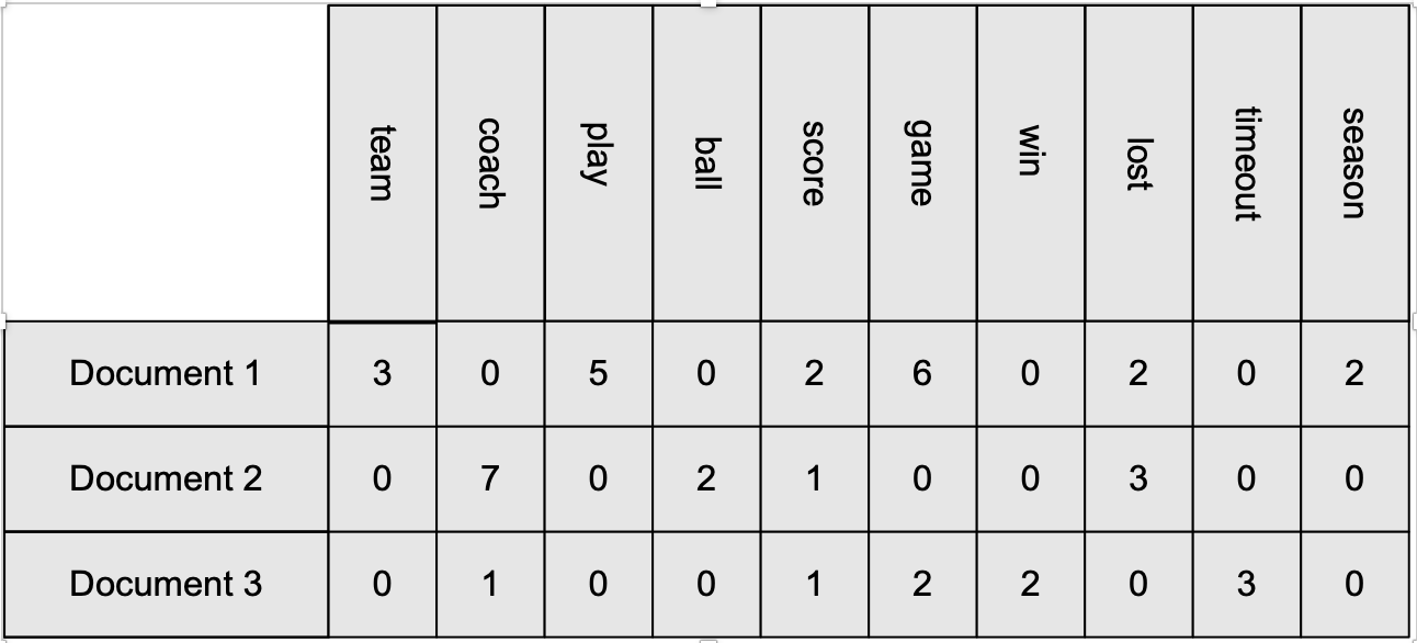
Example of document data where each row represent a document and the columns are set of important words. Each value is the frequency of the that word in the given document.
Transaction Data
A special type of data, where:
- Each transaction involves a set of items.
- For example, consider a grocery store. The set of products purchased by a customer during one shopping trip constitute a transaction, while the individual products that were purchased are the items.
- Can represent transaction data as record data
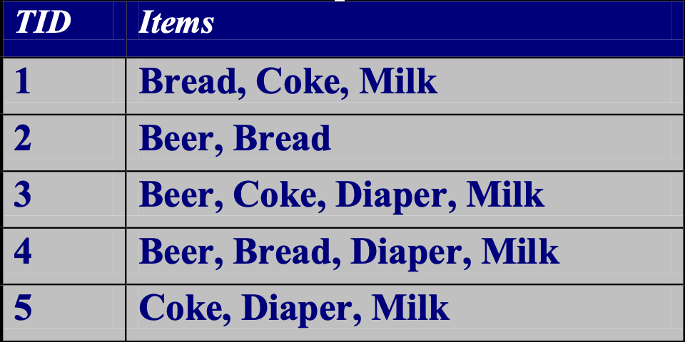
This table represents transaction data, where each row corresponds to an individual transaction. The first column shows the transaction ID, and the second column lists the items included in each transaction
Graph Data
Graph data is a powerful way to represent relationships between entities, capturing connections and interactions in a structured format. For example, in a document network, each node in the graph could represent a document, while the edges represent citations or hyperlinks between these documents, effectively mapping out the interconnections within a body of literature or web pages. Similarly, in the field of chemistry, graph data is used to model molecular structures, where nodes represent atoms and edges represent chemical bonds. This allows researchers to analyze the molecular composition, identify patterns in chemical structures, and predict properties of compounds based on their molecular graphs. The graph representation is particularly useful for visualizing complex relationships and for conducting analyses such as network connectivity, pathfinding, and clustering.
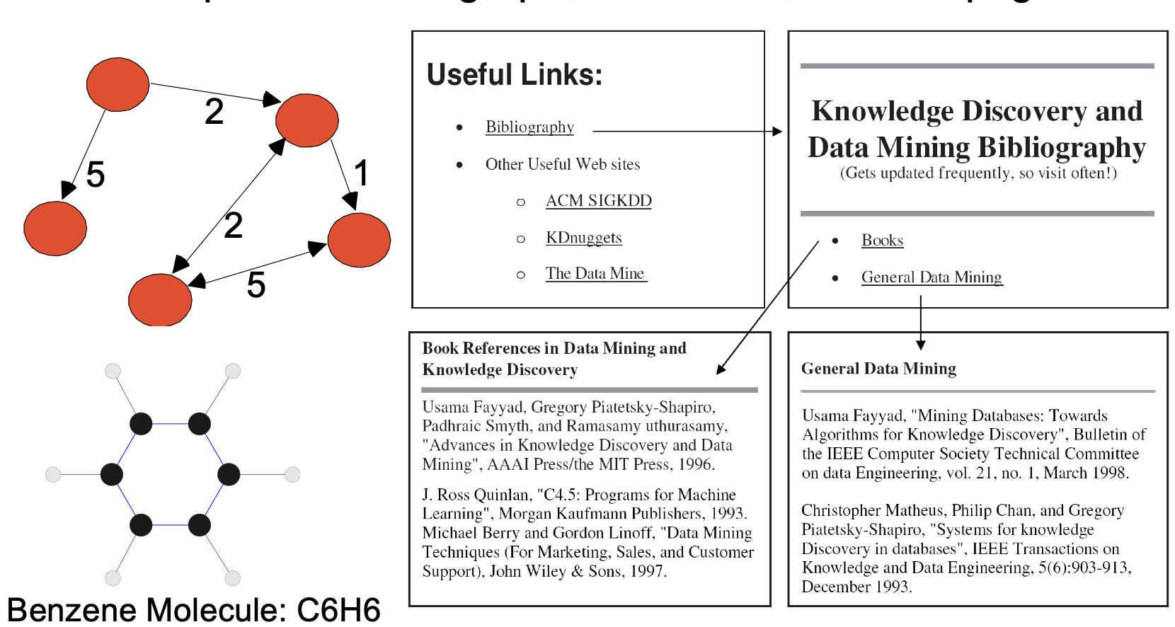
Example of Graph data.
Ordered Data
Ordered data refers to data where the sequence or order of the values is significant. This type of data is commonly encountered in situations where the progression, ranking, or sequence of items carries important information. Ordered data can be found in various contexts, such as time series data, where the order of data points over time is critical for analysis, or in ranked lists where items are arranged based on certain criteria, such as the ranking of students based on their grades.
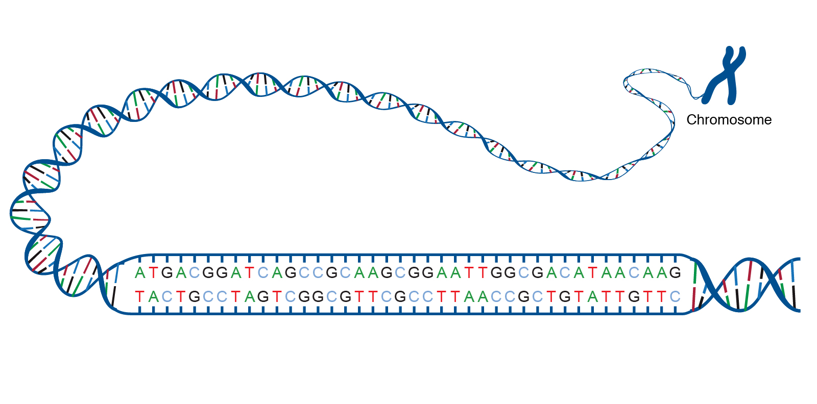
A DNA molecule consists of two strands wound around each other, with each strand held together by bonds between the bases. Adenine pairs with thymine, and cytosine pairs with guanine. The sequence of bases in a portion of a DNA molecule, called a gene, carries the instructions needed to assemble a protein.
Spatio-Temporal Data
Description of Spatio-Temporal Data
Spatio-temporal data refers to data that involves both spatial and temporal dimensions, meaning it includes information about the location and time of events or observations. This type of data is critical for understanding phenomena that change over time and space, such as weather patterns, traffic flow, migration trends, or the spread of diseases.
In spatio-temporal data, each data point typically contains three key components: the location (spatial component), the time at which the event or observation occurred (temporal component), and the attribute or value being measured. This combination allows for a comprehensive analysis of how certain variables evolve in both space and time.
For example, in climate studies, spatio-temporal data might include temperature readings across different geographic locations over several years. Analysts can use this data to track how temperature changes in different regions over time, which is crucial for understanding climate change.
Spatio-temporal data is often represented through maps, animations, or complex models that highlight trends and patterns across both dimensions. The analysis of such data requires specialized techniques that can handle the dynamic nature of the data, taking into account the interactions between the spatial and temporal aspects.
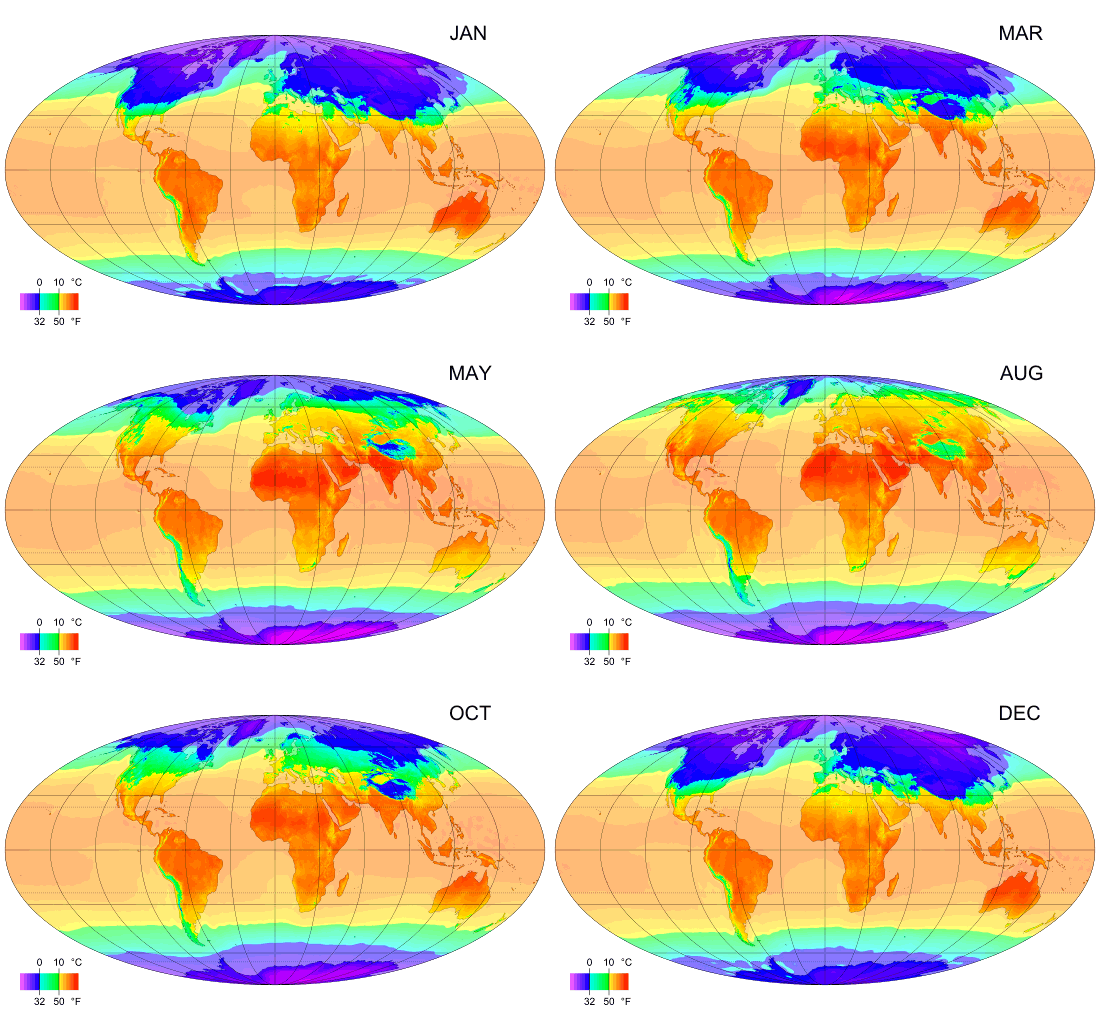
Average Monthly Temperature of land and ocean.
Data Quality
Poor data quality negatively affects many data processing efforts and can lead to significant consequences. For instance, in data mining, if a classification model designed to detect people who are loan risks is built using poor data, the model’s predictions will be unreliable. This could result in credit-worthy candidates being wrongly denied loans, while more loans are given to individuals who are likely to default. These outcomes not only harm the affected individuals but also increase financial risk for the lending institution. Therefore, maintaining high data quality is essential to ensure accurate analysis, reliable predictions, and sound decision-making.
- What kinds of data quality problems?
- How can we detect problems with the data?
-
What can we do about these problems?
- Examples of data quality problems:
- Noise and outliers
- Wrong data
- Fake data
- Missing values
- Duplicate data
Noise
Noise in data can manifest in various forms, depending on whether it affects objects or attributes. For objects, noise is an extraneous object that doesn’t belong to the data set, potentially skewing the results. In the context of attributes, noise refers to the modification of original values, which can distort the data’s integrity and lead to inaccurate analyses.
For example, noise can be seen in the distortion of a person’s voice during a phone call with poor reception or the appearance of “snow” on a television screen. These examples illustrate how noise can obscure or alter the original signal, making it difficult to interpret correctly.
The figures below illustrate this concept with sine waves: two sine waves of the same magnitude but different frequencies are shown, first individually, then combined, and finally with added random noise. The introduction of noise distorts the magnitude and shape of the original signal, demonstrating how noise can significantly affect data quality and clarity.

Example of noise affecting the quality of the data. In the left, we have the representation of two sinus waves. In the middle their sum and on the right we see the effect of noise on the transmitted signal.
Outliers
Outliers are data objects with characteristics that are significantly different from most other data objects in a data set. These anomalies can either interfere with or be the focus of data analysis, depending on the context.
-
Case 1: Outliers as noise – In many analyses, outliers can act as noise, disrupting the accuracy of the results and leading to misleading conclusions. These outliers might need to be removed or treated carefully to ensure the integrity of the analysis.
-
Case 2: Outliers as the goal of analysis – In other scenarios, outliers are the primary target of the analysis. For example, in credit card fraud detection, unusual transactions (outliers) are flagged for further investigation. Similarly, in intrusion detection systems, identifying outliers can help in detecting unauthorized access or attacks.
Understanding the nature of outliers and their impact is crucial for effective data analysis, as they can either distort the results or reveal critical insights.
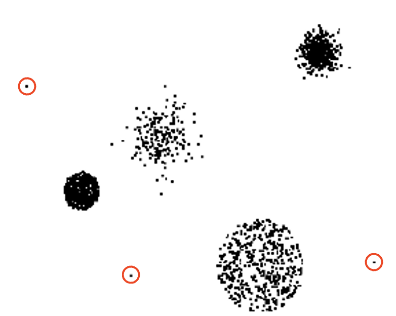
Example of outliers data that interfere with the data analysis.
Missing Values
Missing data in a dataset can arise due to various reasons, and it presents unique challenges for analysis.
Reasons for Missing Values
- Information is not collected: In some cases, certain data might be missing because it was not collected. For example, individuals might decline to provide sensitive information such as their age or weight.
- Attributes may not be applicable to all cases: Sometimes, certain attributes are irrelevant for specific cases. For instance, the attribute “annual income” would not be applicable to children, leading to missing values for this attribute in a dataset that includes both adults and children.
Handling Missing Values
- Eliminate data objects or variables: One approach to dealing with missing data is to remove the data objects (rows) or variables (columns) that contain missing values. This method, however, can lead to loss of information.
- Estimate missing values: Another approach is to estimate and fill in the missing values using techniques like interpolation in time series data, or using demographic averages in census data.
- Ignore the missing value during analysis: In some cases, it may be feasible to simply ignore the missing values during analysis, depending on the method being used and the amount of missing data.
Handling missing data effectively is crucial for ensuring the accuracy and reliability of data analysis results.
| Name | Date of Birth | Gender | Annual Income |
|---|---|---|---|
| John Doe | 1985-06-15 | Male | $50,000 |
| Jane Smith | Female | $65,000 | |
| Tom Brown | 1990-02-28 | Male | |
| Lisa White | Female | $70,000 |
