Classification with Naives Bayes

Naive Bayes models are a group of extremely fast and simple classification algorithms that are often suitable for very high-dimensional datasets. Because they are so fast and have so few tunable parameters, they end up being very useful as a quick-and-dirty baseline for a classification problem. This homework will focus on an intuitive explanation of how naive Bayes classifiers work, followed by a couple examples of them in action on some datasets.

Bayesian Classification

Naive Bayes classifiers are built on Bayesian classification methods. These rely on Bayes’s theorem, which is an equation describing the relationship of conditional probabilities of statistical quantities. In Bayesian classification, we’re interested in finding the probability of a label given some observed features, which we can write as P(L |features) . Bayes’s theorem tells us how to express this in terms of quantities we can compute more directly:

If we are trying to decide between two labels—let’s call them $L_1$ and $L_2$ —then one way to make this decision is to compute the ratio of the posterior probabilities for each label:

Gaussian Naive Bayes

Perhaps the easiest naive Bayes classifier to understand is Gaussian naive Bayes. In this classifier, the assumption is that data from each label is drawn from a simple Gaussian distribution.

Let’s start with by creating a blobs that will serve as our dataset.

1
2
3
4
5
%matplotlib inline
import numpy as np
import matplotlib.pyplot as plt
import seaborn as sns; sns.set()

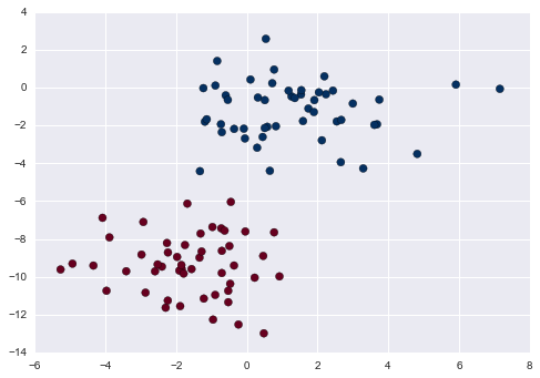
We will the the make_blobs from sklearn.datastet to create a dataset with two classes (centers) and will to learn how to classify them.

1
2
3
from sklearn.datasets import make_blobs
X, y = make_blobs(100, 2, centers=2, random_state=2, cluster_std=1.5)
plt.scatter(X[:, 0], X[:, 1], c=y, s=50, cmap='RdBu');

This will produce the following plot.

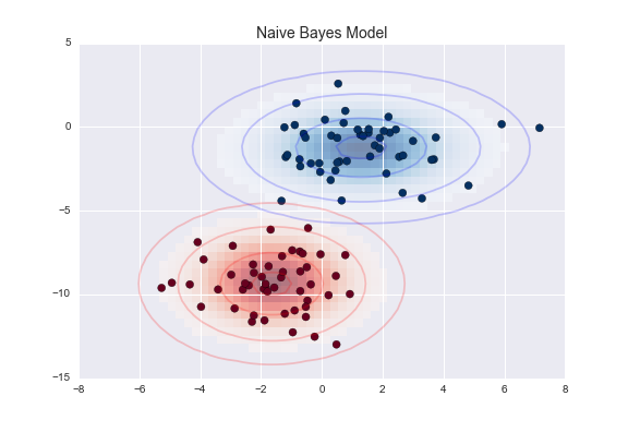
One extremely fast way to create a simple model is to assume that the data is described by a Gaussian distribution with no covariance between dimensions. This model can be fit by simply finding the mean and standard deviation of the points within each label, which is all you need to define such a distribution. The result of this naive Gaussian assumption is shown in the following figure.

Let’s try to classifiy this data using Naive Bayes.

1. First create a Naive Bayes classifier from the sklearn library.
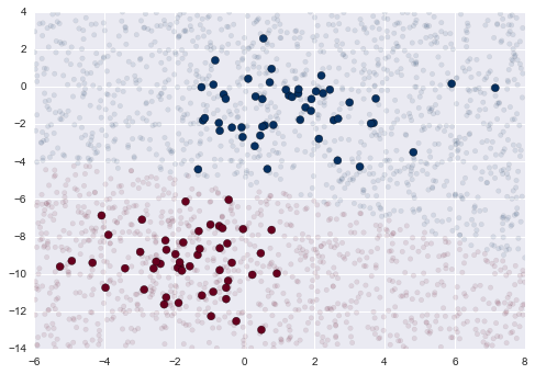
2. Show the decision boundary by prediting the class of a set of points. Try to produce the following plot.

1. You should generate a set of points in the shown box.
2. For each point color the point given the classification for your naive bayes.
3. Plot the data.

We see a slightly curved boundary in the classifications—in general, the boundary in Gaussian naive Bayes is quadratic.

Multinomial Naive Bayes

The Gaussian assumption just described is by no means the only simple assumption that could be used to specify the generative distribution for each label. Another useful example is multinomial naive Bayes, where the features are assumed to be generated from a simple multinomial distribution. The multinomial distribution describes the probability of observing counts among a number of categories, and thus multinomial naive Bayes is most appropriate for features that represent counts or count rates.

The idea is precisely the same as before, except that instead of modeling the data distribution with the best-fit Gaussian, we model the data distribuiton with a best-fit multinomial distribution.

Classifying text.

Here we will use the sparse word count features from the 20 Newsgroups corpus to show how we might classify these short documents into categories.

Let’s download the data and take a look at the target names:

1
2
3
4
from sklearn.datasets import fetch_20newsgroups

data = fetch_20newsgroups()
data.target_names

1
2
3
4
5
6
7
8
9
10
11
12
13
14
15
16
17
18
19
20
['alt.atheism',
 'comp.graphics',
 'comp.os.ms-windows.misc',
 'comp.sys.ibm.pc.hardware',
 'comp.sys.mac.hardware',
 'comp.windows.x',
 'misc.forsale',
 'rec.autos',
 'rec.motorcycles',
 'rec.sport.baseball',
 'rec.sport.hockey',
 'sci.crypt',
 'sci.electronics',
 'sci.med',
 'sci.space',
 'soc.religion.christian',
 'talk.politics.guns',
 'talk.politics.mideast',
 'talk.politics.misc',
 'talk.religion.misc']

For simplicity here, we will select just a few of these categories, and download the training and testing set:

1
2
3
4
categories = ['talk.religion.misc', 'soc.religion.christian',
              'sci.space', 'comp.graphics']
train = fetch_20newsgroups(subset='train', categories=categories)
test = fetch_20newsgroups(subset='test', categories=categories)

In order to use this data for machine learning, we need to be able to convert the content of each string into a vector of numbers. For this we will use the TF-IDF vectorizer, and create a pipeline that attaches it to a multinomial naive Bayes classifier:

1
2
3
4
5
6
from sklearn.feature_extraction.text import TfidfVectorizer
from sklearn.naive_bayes import MultinomialNB
from sklearn.pipeline import make_pipeline

model = make_pipeline(TfidfVectorizer(), MultinomialNB())

Question 2:

1. Train the predifined model.
2. Print the confusion matrix for for the classification error.
3. Now let’s have some fun and use our model to predict the classes for a given clauses:
4. sending a payload to the ISS
5. discussing islam vs atheism
6. determining the screen resolution