Decision Tree Classification

Introduction to Decision Tree Classification Using the Titanic Dataset

In this homework, you will explore the decision tree classification method using the famous Titanic dataset. Your objective is to predict whether a passenger in the test set survived based on available features. Through this assignment, you will learn how to analyze the dataset, handle missing values, and understand the impact of different decision tree parameters, such as criteria and tree depth. Additionally, you will use the dtreeviz package to visualize the decision-making process of the tree, which will help in interpreting and refining your model’s predictions.

Set up

You will work on building a decision tree classifier to predict whether a passenger on the Titanic survived, based on various features in the dataset. To begin, please download the Titanic dataset from Kaggle’s Titanic - Machine Learning from Disaster competition. The dataset consists of three main files:

1. train.csv - The training data with labeled outcomes (Survived column).
2. test.csv - The test data without labeled outcomes, used for making survival predictions.
3. gender_submission.csv - A sample submission file showing the expected format for predictions.

After downloading the files, you will start by investigating the data, handling missing values, and exploring different decision tree parameters (such as depth and criterion) to optimize your model. Additionally, you’ll use the dtreeviz package to visualize the decision-making process of your tree, helping you understand the classification path for each prediction.

If you’re using the kaggle API, you can download the files with

1
kaggle competitions download titanic

Start a new netebook and add the following two cells to prepare teh notebook

1
2
3
4
import numpy as np
import matplotlib.pyplot as plt
import pandas as pd
import dtreeviz   # pip install dtreeviz

and prepare matplotlib.

1
2
3
%config InlineBackend.figure_format = 'retina' # Make visualizations look good
#%config InlineBackend.figure_format = 'svg' 
%matplotlib inline

Question 1: Load and Summarize Missing Data

1. Begin by loading the train.csv and test.csv files into your environment. Use the pandas library to read these files as dataframes.

2. Once loaded, print a summary of the missing data for each column in both datasets. To accomplish this, use the .isna() function combined with .sum(), which will show the total count of missing values in each column.

   Hint: You can apply .isna() to your dataframe to get an overview of which columns have missing data and how much data is missing in each.

Question 2:

As you can see, the column Cabin is almost empty, so we will drop it (not use this columns). But for the column Age we could fill the missing data by the mean.

1. Use the function drop to remove the Cabin column.
2. Use the function fillna to replace the missing data in the Age column with the mean.
3. Also use the drop method to remove the name as it not relevant to decide if the passenger has survived or not.

Question 3:

The dataset still contain some Categorical variables that need to be encoded.

1. Identify those columns.
2. Transform those column as the type category and use the cat.codes to get their codes.

Question 4: Decision Tree Classifier

1. Now declare a list called features that will hold the features that you see fit to decide if the passenger have survided.
2. Name the target column with Survived
3. Import the classifier which is in sklearn.tree.DecisionTreeClassifier
4. for the first time we will take all the values by default.
5. Train the model on the choosen data. For this read the documentation for the fit function.

Question 5: Accuracy and confusion matrix

Now we move to evaluate the accuracy of our vanilla model ( with the basic default argument). We will use two tools to evaluate the performance of our decision tree.

1. Accuracy.
2. Confusion matrrix

Accuracy

The accuracy of the model is simply the percentage of correct labeled class over the dataset

[ \text{accuracy} = \dfrac{P}{N} ]

Where $P$ is the number of correct instances that are correclty labeled. and $N$ is the size of the dataset.

Search the moduls sklearn.metrics for this function

The values you got are the accuracy on the train datast. In order to measure the performance of our model, we can evaluate this metric on kaggle Titanic. You will get about 75% score which is not bad for a single Tree decision.

Now we move to the confusion score which will save the state for our four classes:

• TP: number of instances in the dataset with the true label that were correcly identified.
• FP: Number of instances in the dataset with the false label thar were wrongly labeled as True.
• TN: Number of instances in the dataset with the false label that were correctly identified as False.
• FN: Number of instances in the dataset with the True label that were wrongly labeled as False.

the confusion matrix will plot the following matrixx

Sear this function in the sklearn.metrics and compute those values on the training set.

Question 6:

The goal of the next section is to see the effect of choosing the Criterion on the overal test accuracy and training accuracy.

Try to change the criterion in the function and compute the training accuracy for the following criterias:

• gini
• entropy
• log_loss

which criterion gives the best accuracy on the test data?

Quesiton 7:

Another hyper-parameter to choose is the depth of the tree. You can choose this parameter by

• max_depth : which represent the maximal height of the tree.
• min_samples_split : which represents the minimal height for the tree.

What are the best values you got by modifying this parameter?

Question 8:

Now we move to visualize the key elements on the decision for our classifier.

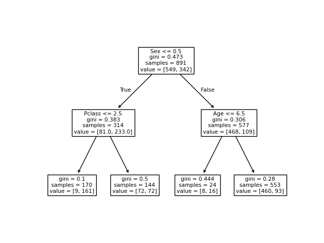
Use the sklearn.tree.plot_tree to show how the decision process is completed for each instance.

For better understanding try to minimize the max_depth of the tree

You will get a picture like this:

Question 9:

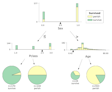
Now we move to a more advanced visualisation. We will use the

1. dtreeviz Try to install the package by

   1
   pip install dtreeviz
   

2. In order to the package to work you also need to install the GraphVis

Use the following code to visualize the tree.

1
2
3
4
5
6
7
8
9
10
# Visualizing the tree
viz_model = dtreeviz.model(tree_classifier,
                           X_train=X_train, y_train=y_train,
                           feature_names=features,
                           target_name=target, class_names=["perish", "survive"])

# getting the view
v = viz_model.view()
v.show()
plt.show()

That will a plot explaining the process for the decision tree with a max level 2.

Question 10:

Now you’re able to use a decision Tree classifier and plot the decision process. You could also plot the decision areas for datasets with only ttwo features. In order to that, try to reproduce the same work on the Iris dataset. You can load the dataset using the sklearn package by

1
from sklearn.datasets import load_iris

Once you have prepared your classifier, you can visualize the classes by

1
2
3
4
5
viz_model = dtreeviz.model(dtc_iris,
                           X_train=X, y_train=y,
                           feature_names=features,
                           target_name='iris',
                           class_names=class_names)

and

1
viz_model.ctree_feature_space(show={'splits','title'}, features=['petal length (cm)', 'petal width (cm)'])